Designing a loudspeaker with LoudspeakerLab
This guide explains LoudspeakerLab’s tools, why its design calculations do not use trained AI, and the science behind the results.
Start with the driver data, then work through the cabinet and crossover before judging the finished curves. The chapters below follow those decisions and show the controls you will use along the way. Equations are included where they help explain a result, with longer derivations kept in expandable sections. Section 12 collects the Frequently Asked Questions on uploads, calibration, enclosure options, solver behavior, account access, and display preferences. The comparison in Section 11 is useful when you need to decide which design tool suits a particular job.
The guide covers full-wave 3D Boundary Element Method (BEM) and edge-diffraction modeling across closed cabinets, coupled chambers, stacked multi-module towers, open panels, hybrid panel-over-box constructions, and measured assemblies. Crossovers can be passive, active, or a combination of the two, with IIR or FIR processing where the selected device supports it. Auto-Solve can develop supported passive, active, and hybrid arrangements, while the editor lets you adjust the circuit, wiring groups, and channel filters yourself. The geometry, measurement basis, and hardware limits still matter, so check the relevant chapter before choosing a layout around a feature.
Contents
Reading the equations
A transfer function is output divided by input at each frequency. A complex number keeps both level and phase, so the calculation can distinguish waves that add from waves that cancel. In the equations, $f$ is frequency in hertz, $\omega=2\pi f$, and $j=\sqrt{-1}$. The DSP sample rate is $F_s$, while the driver’s free-air resonance is $f_s$. Pressure level changes by $20\log_{10}$ of a pressure ratio, and power level changes by $10\log_{10}$ of a power ratio. An octave doubles the frequency. Phase describes a wave’s position in its cycle, polarity reverses its sign, and delay moves it in time.
1. What you can do in LoudspeakerLab
LoudspeakerLab combines driver measurements, enclosure simulation, cabinet radiation, and crossover design in a browser. A project keeps these inputs together so you can see how a change to the cabinet or crossover affects the predicted response. The models serve different purposes. Thiele-Small parameters describe low-frequency driver and enclosure behavior. Measured response and impedance curves describe the driver over a wider frequency range. The crossover calculation applies electrical and digital filtering, while the cabinet and acoustic calculations couple each radiator to its enclosure, baffle, and listening geometry.
A useful design needs more than a flat on-axis response. Check the listening window, off-axis response, impedance, and estimated output limits together. A change that improves one curve can make another worse. For example, extra attenuation can smooth a handoff while reducing the available output.
1.1 Find the tool you need
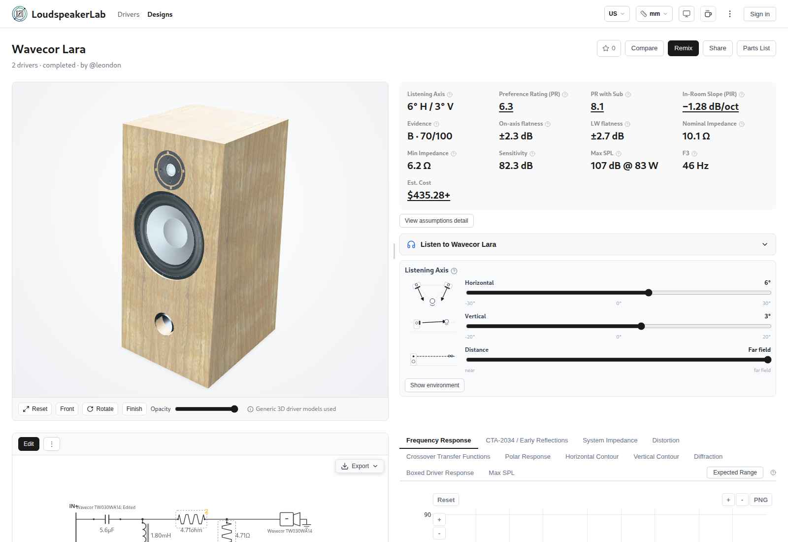
You can browse public driver profiles and designs before signing in. Sign in to upload measurements, create and save drafts, or remix a published design. A new design starts with two steps. Choose the drivers first, then review the cabinet. The completed draft opens in the crossover editor.
| Task | What you can do | Where it is explained |
|---|---|---|
| Find and compare drivers | You can filter canonical driver models by cost, size, usable band, specifications, and evidence. You can compare curves, check cost-per-value context, and choose a measurement profile for each model. | Section 3.7 |
| Add driver data | You can upload response, impedance, distortion, and near-field files, prefill catalog defaults, import spec-sheet text, and accept or override the automatic open-or-sealed rear suggestion. | Section 3.11 |
| Choose the bass enclosure | You can size sealed, vented, and passive-radiator enclosures, select prebuilt commercial cabinets, and inspect bass response, cone travel, group delay, port speed, and fast Box Review acoustic previews. | Section 4 |
| Lay out a cabinet | You can configure five cabinet shapes (rectangular, tapered-shoulder, arched-top, stepped-baffle, and stacked modules), front and rear rake, free-standing or in-wall placement, ports, edge treatments, and chamber or panel construction. | Section 4.6 |
| Inspect cabinet radiation | You can inspect full-wave 3D BEM and Svensson edge-diffraction cabinet radiation, coupled multi-aperture loading, full ±180° contours, and 3D radiation globes in the read-only Cabinet Effect view. | Section 5.0 |
| Edit a passive crossover | You can edit series, shunt, and parallel networks, combine same-model siblings into parallel or series wiring groups, split high-dissipation resistors, and import or export SPICE text or portable complete netlist bundles. | Section 6 |
| Search for a crossover | Auto-Solve searches supported passive arrangements and develops active or hybrid filtering within the saved amplifier-channel layout while preserving driver order and branch identities. | Section 9 |
| Design an active or hybrid crossover | You can assign amplifier channels across 14 device profiles, edit gain, delay, EQ, crossover, all-pass, and FIR blocks, apply endfire cardioid presets, and export native setups or manual parameter sheets. | Section 6.4 |
| Judge the acoustic response | You can inspect individual driver responses, their sum, phase, crossover transfers, distortion data, polar plots, contours, far-field CTA-2034 curves, and coverage fade beyond measured frequency bands. | Section 7 |
| Change the listening position | You can inspect a finite-distance Listener point separate from standardized far-field curves, view an expanding 3D radiation balloon, and open mobile WebXR or iOS gyroscope AR views. | Section 7.2 |
| Check output and amplifier load | You can inspect impedance magnitude and phase, estimated maximum SPL, excursion limits, and component heating across passive, coupled, directional, and multi-channel active designs. | Section 8 |
| Check the basis of a prediction | On-demand Expected Range on response, CTA-2034, and impedance plots, along with evidence scores, assumptions detail, and design-local source assumptions, explain the data basis and sensitivity. | Section 10.2 |
| Compare and listen | You can compare completed designs and listen to a filtered-noise demonstration of their frequency balance. | Section 10.5 |
| Prepare a build | You can review parts matched across 12 component and 11 driver vendors in five regions with bulk cart links where supported, build and cut sheets, PBR finishes with ambient occlusion, and mobile AR placement. | Section 4.7 and Section 10.4 |
| Save and share your work | You can save an editable draft, fork a published crossover, migrate a published design to a replacement driver, publish a fixed public version, remix designs, and post stars or comments. | Section 10.6 |
For a first design, follow the five-step workflow in Section 10.1. Keep the driver profiles, cabinet, and listening settings fixed while comparing crossover changes. If you change the cabinet, check its bass loading and driver positions again before judging the new result. Save a useful revision so you have a clear reference for the next edit.
1.2 Frequency grid and acoustic reference
Final analysis normally uses 48 points per octave on a logarithmic grid. Each step represents the same frequency ratio, rather than the same number of hertz. This gives the bass and treble comparable resolution when viewed in octaves. The formula below sets those sample frequencies from the chosen points per octave.
At 48 points per octave, the grid has 480 samples from 20 Hz to about 20,186 Hz. The final sample extends beyond 20 kHz to keep the spacing uniform. Search stages can use lower resolutions. Stored measurement files keep their own acquisition grids, and the live Box Review perimeter preview uses an 81-point grid for immediate feedback.
The core response is an anechoic prediction. It does not include the reflections or room modes of a particular listening room. The predicted in-room curve in Section 7 is a weighted summary of radiation in different directions. It does not simulate your room.
1.3 What the controls change
LoudspeakerLab follows a consistent physical sequence from driver measurements to finished system curves. First, each driver's response and impedance are normalized to a common reference and stripped of known measurement-cabinet effects so box and baffle loading are never counted twice. Next, physical chambers, enclosure alignments, and prepared cabinet or panel radiation models compute how the drivers and any ports or passive radiators load and radiate into free air. Finally, channel DSP, passive crossover circuits, wiring groups, and 3D driver locations combine as complex pressures to produce the system curves and output-limit checks.
Choose the drivers and their measurement profiles before setting out the cabinet or panel. Place the sources, check the listening reference, and decide how they will share amplifier channels or passive wiring groups. You can then enter a crossover yourself or use Auto-Solve to develop a supported layout. Each driver retains a stable branch identity across edits, reorders, and Auto-Solve runs, keeping twin drivers distinct across every plot legend. Read the response, directivity, amplifier loads, output limits, and parts together before saving a revision.
The units setting changes how cabinet dimensions and volumes are shown. The region setting changes currency, regional pricing, and local shopping links. Neither changes the underlying physics. Saving a design stores its chosen settings and completed result. While editing a crossover, a fast preview updates immediately in your browser, and the authoritative calculation settles automatically shortly after you pause.
1.4 Read the plots
Frequency runs from left to right. Equal distances represent equal frequency ratios, so the space from 100 to 200 Hz is the same as the space from 1 to 2 kHz. The vertical scale often shows sound-pressure level in decibels. Check its label and reference before comparing plots. Where a calculation extends beyond a driver's measured frequency or angular range, preview curves fade to half opacity so extrapolated regions remain visually distinct from measured data.
Hover over a curve to read its value. Use the legend to hide or show traces, zoom to inspect a band, and select Reset to restore the view. The PNG control saves an image of the plot. A normalized contour shows how level changes with direction. Its colors do not necessarily represent the absolute SPL at a listening seat.
2. Why LoudspeakerLab does not use AI for design calculations
LoudspeakerLab uses physical calculations and numerical search for its design results. That includes passive, active, and hybrid crossovers, enclosure design, coupled cabinet radiation, system response, impedance, and output-limit estimates. Driver measurements, circuit values, cabinet geometry, and operating assumptions supply the inputs to those calculations. Auto-Solve compares candidates using their calculated behavior rather than a trained model's prediction of a finished design.
You can inspect the measurements, circuit, filters, and assumptions behind a result. Changing a component or channel setting runs the relevant calculation again for that design. LoudspeakerLab has not adopted a trained predictor whose accuracy is established across the combinations of inputs and outputs these features require. The reasons for that choice are described below, along with the limits of the physical models.
2.1 What powers the features that can look like AI?
| LoudspeakerLab feature | Inputs used | Calculated result |
|---|---|---|
| Auto-Solve | Driver response and impedance, cabinet, listening context, channel layout, DSP device where used, and your priorities and constraints. | A supported crossover, including passive parts or channel IIR/FIR processing, evaluated with the final values and coefficients. |
| Box design | Driver parameters, enclosure type, volume, tuning, losses, and relevant port or radiator settings. | Predicted bass response, cone motion, coupled cavity loading, and port or radiator behavior under the chosen assumptions. |
| System response and directivity | Driver measurements, phase, positions, 3D BEM and edge-diffraction cabinet or panel radiation, crossover filtering, and listening direction. | Combined complex sound-pressure response, phase, far-field CTA-2034 curves, finite-distance listener response, and angular summaries within the supported model's coverage. |
| Impedance and amplifier load | Driver impedance, enclosure and coupled-aperture loading where applicable, component values and losses, wiring, and channel assignments. | Impedance magnitude and phase over frequency, combined for the appropriate amplifier load. |
| Thermal handling and output limits | Driver ratings and excursion limits, crossover transfer functions, component ratings, signal assumptions, and amplifier limits. | Estimated component dissipation, mechanical and thermal limits, and maximum SPL where sufficient inputs are available. |
For thermal handling, LoudspeakerLab calculates electrical stress and applies the stated ratings and signal assumptions. It does not model changing voice-coil temperature feeding back into the response. These are estimates with declared limits, as explained in Section 8. A resistor rating and a driver power rating describe different limits, even when both are expressed in watts.
2.2 The missing training basis: complete inputs matched to complete outputs
A trained replacement for these calculations would need many matched examples of a complete design and its corresponding behavior. The inputs would have to include the driver parameters and measurements, cabinet and loading, complete circuit, component losses, listening geometry, and relevant operating conditions. The outputs would have to include the resulting system response, phase and directivity, impedance, excursion, component dissipation, and thermal or output limits. An active example would also need the actual channel routing, device rate, and filter coefficients used for the corresponding measurements.
Individual driver profiles are not a training set of complete loudspeaker outcomes. A measured driver response does not label what every crossover and cabinet combination will produce. A circuit diagram does not supply the corresponding measured angular response, impedance, and power handling. Even a published design can omit the timing reference, exact measurement conditions, component losses, or high-level behavior needed to make that example usable for training.
LoudspeakerLab therefore has no trained predictor for these features whose accuracy has been established across its supported driver, enclosure, and circuit combinations. Supplying driver data to a general language model does not train or validate such a predictor. A model's familiarity with driver names or common crossover recipes does not establish the required relationship between complete inputs and outputs. Those calculations remain necessary when an unfamiliar driver or channel arrangement is introduced.
Training on results generated by LoudspeakerLab's own calculations would create an approximation to those calculations. It would still need independent error checks across the supported design space, and it would inherit the underlying model's omissions. Such training would not supply missing measurements or establish real thermal behavior. LoudspeakerLab currently evaluates the physical model directly.
2.3 Why a plausible AI answer is insufficient for these features
The outputs are coupled. A component change alters filtering and amplifier load through the driver's frequency-dependent impedance. Phase and driver spacing affect whether the acoustic outputs add or cancel. Box volume and tuning affect bass response and excursion. Component dissipation and driver limits depend on the resulting electrical drive and the assumed signal.
A useful prediction must preserve these relationships on the same candidate. Small errors near a resonance, crossover null, or minimum impedance can change the design decision. A learned model would need validation of those cases and of unfamiliar combinations, including phase and electrical limits, before LoudspeakerLab could rely on its outputs. A language model can also give a confident but incorrect explanation or set of component values, a risk described in NIST's generative AI profile. LoudspeakerLab needs calculated curves and constraints that can be inspected for the selected design. This is why generated circuit or box recommendations are not the basis of its design results.
2.4 Why computational search and differential evolution were chosen
Physical evaluation gives LoudspeakerLab a way to test a proposed circuit against explicit goals using the actual project inputs. Computational search compares supported circuit arrangements. Numerical optimization adjusts their values and evaluates the consequences. This approach can work with a new combination of supported drivers and parts without a training example of that finished speaker.
Differential evolution is useful for crossover tuning because several component values interact and the response can have multiple promising regions. It explores sets of values and uses differences between candidates to propose alternatives, keeping useful improvements. It does not require derivatives of the objective or a trained prediction model. Storn and Price's original paper describes the general numerical method.
LoudspeakerLab chose this approach so alternatives can be compared on the modeled acoustic and electrical behavior under your chosen priorities and constraints. The search can investigate circuit arrangements as well as values. The selected result remains an inspectable circuit with final parts and calculated curves. Section 9 explains Auto-Solve's controls and results.
Box design uses enclosure equations and alignment targets, with numerical fitting where a measured curve must be matched. It does not need to learn box behavior from completed designs. Differential evolution is part of the crossover search and is not required for every enclosure calculation. System response, impedance, and output-limit estimates likewise use their appropriate physical relationships and stated assumptions.
Evolutionary methods are sometimes grouped under the broad term AI. In this discussion, the distinction concerns trained models that generate a design or predict its engineering outputs. LoudspeakerLab's search uses numerical evaluation and explicit goals. It does not train a neural model of the speaker.
2.5 What this choice means for your results
You can inspect the inputs, circuit, assumptions, and outputs, then recalculate the effect of an edit. Computational search takes evaluation work and can return different candidates on different runs. It does not prove a global optimum or guarantee that every goal is met. Keep useful candidates as separate revisions so their circuits and curves can be compared.
Physical models also have limits. Incorrect driver data, missing measurements, uncertain ratings, or geometry outside the model's accepted range can produce a poor prediction. LoudspeakerLab's choice of numerical design makes those dependencies visible. Prototype measurements remain necessary to establish how the assembled speaker behaves.
3. Driver Measurements and Parameters
Start with the driver profile. Check the source of the curves, the measurement conditions, and the available frequency range before using the driver in a design. A curve traced from a datasheet and a calibrated laboratory measurement can look similar on screen, but they do not provide the same evidence. Choose the measurement profile before entering the cabinet dimensions or a crossover target.
3.1 Thiele-Small Parameters
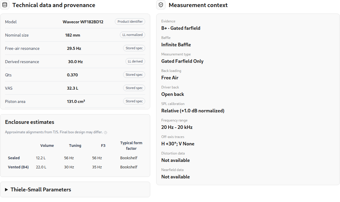
Thiele-Small parameters describe the driver's small-signal behavior near resonance. The enclosure model uses values such as free-air resonance $f_s$, total quality factor $Q_{ts}$, and equivalent compliance volume $V_{as}$, while cone area $S_d$, linear excursion $X_{\max}$, and rated power support output-limit estimates. Resonance $f_s$, $Q_{ts}$, and $V_{as}$ are required for open-backed non-planar drivers that load an enclosure, whereas sealed-back and planar drivers retain those parameters when supplied without requiring them. Supplied parameters are checked against physical sanity bounds ($f_s$ from 5 to 3,000 Hz, $R_e$ from 0.5 to 100 ohms, $Q_{es}$ from 0.05 to 10, $Q_{ms}$ from 0.2 to 100, and $L_e$ up to 20 mH).
LoudspeakerLab never overwrites values you enter, and it fills missing physical parameters non-destructively when enough supporting data exist. It can estimate $S_d$ from frame diameter, complete $Q_{ts}$ from $1/Q_{ts} = 1/Q_{es} + 1/Q_{ms}$, derive $L_e$ from impedance data, and estimate $V_{as}$ from regression or fit free-air resonance and quality factors from a free-air impedance curve. In-box impedance measurements skip free-air parameter extraction because the enclosure alters the resonance. As with any single-curve fit, a single free-air impedance sweep cannot independently determine every mechanical parameter such as $V_{as}$ without supporting box or mass data.
3.2 Measurements Taken in a Box
A vented test box produces two impedance peaks with a minimum near the port tuning frequency. LoudspeakerLab can fit a box-loaded impedance model when the enclosure information and required driver parameters are available. The fit estimates selected unknowns and reports diagnostics. Check the fitted curve against the measurement. A close fit is useful evidence, but it does not prove that each fitted parameter is unique. Incorrect box volume, incomplete low-frequency data, and unmodeled losses can affect the result.
3.3 Impedance in the Target Enclosure
Changing the enclosure changes the driver's low-frequency impedance. A sealed box shifts its resonance, while a vented box introduces the two-peak pattern associated with its tuning. The model estimates the motional impedance of the measurement setup and replaces it with the target box contribution. That loaded curve is the impedance seen by the crossover calculation.
The measured high-frequency impedance remains part of the curve rather than being replaced with an ideal inductor. It can include features that a simple lumped model would miss. The source fit and conditioning still affect the loaded result, so not every measured sample is preserved exactly. Inspect the resonance region as well as the upper-band load before choosing the passive filter values.
3.4 Frequency Response and Minimum Phase
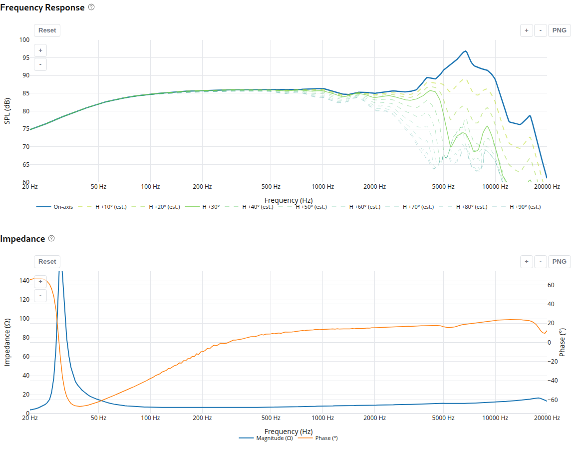
FRD files contain frequency-response measurements, and ZMA files contain impedance measurements. Common two-column and three-column text formats are accepted. When supplied, the third column carries phase. Check the imported curves and units before proceeding. Below a measurement's lowest measured frequency, rolling-off response curves extrapolate at a bounded slope for up to two octaves and then hold flat, applied identically across catalog previews and design calculations so stored archives and live curves stay consistent.
Near-field bass measurements can be merged with gated far-field response. For a vented enclosure, cone and port measurements need the correct relative scaling. The merge uses a smooth transition around the selected splice region. An open panel needs a different bass reference because a cone measurement does not capture cancellation around the panel.
Routine modeled designs use the minimum-phase response implied by the measured magnitude. The calculation converts decibels to log pressure magnitude, places the values on an equally spaced frequency grid, and mirrors the spectrum. An inverse Fourier transform produces the real cepstrum, whose time-zero term is retained and whose positive-time terms are doubled. Transforming that causal cepstrum back gives the minimum-phase angle. Flight time is removed only when recorded as present, acquired phase is retained without being overwritten on measured assemblies, and minimum-phase reconstruction never claims acquired excess phase or removes reflections in magnitude data. For a target assembly with measured timing, use the declared measured-source route described in Section 3.10.
3.5 Phase and Acoustic Center
Relative phase determines how drivers add through the crossover region. Measurements taken with different timing references can create misleading cancellations. LoudspeakerLab therefore matches a shared timing reference automatically across drivers instead of relying on manual timing groups. Drivers share an acoustic timing frame when every measured driver in the group declares a common loopback or acoustic timing reference, uses the same reference method, was measured on the same baffle at the same microphone distance, and keeps acoustic-center offsets within 50 mm.
When a shared reference is missing, or when measured-phase and minimum-phase driver profiles are mixed without reconciliation, LoudspeakerLab does not invent an unverified coherent sum. Instead, it falls back to minimum-phase modeling with geometric acoustic-center priors or blocks the unverified mixed pair until the phase basis is clarified. LoudspeakerLab selects acoustic-center depth from an explicit profile value, an accepted on-axis passband estimate, or a shallow-tweeter versus deeper-cone geometric estimate, avoiding any automatic delay that would double-count timing already present in measured phase. Because an excess-phase slope alone cannot separate microphone distance error from physical center depth without a known reference, a prototype measurement around the intended handoff remains the best check.
3.6 Off-Axis Response
For an axially symmetric driver, including profiles where symmetry is left unspecified and defaults to axially symmetric, one polar family describes the response around its axis. A combined horizontal and vertical direction is therefore reduced to its total angle from that axis. Equal total angles use the same polar response, even if their horizontal and vertical components differ. The relation below gives that angle without treating two independent plane cuts as a full spherical measurement.
A driver with distinct horizontal and vertical families is treated differently. Its two measured plane ratios are multiplied relative to the on-axis response. This reproduces each supplied plane when the other angle is zero. The equation below describes that separable approximation for directions between the planes.
This reproduces the supplied plane cuts, and rear-hemisphere unfolding protects measured vertical polar curves from abrupt meridian jumps. The response between those planes remains an approximation because two plane cuts do not contain the same information as a measured spherical dataset. Where angular measurements are missing, directivity completion can estimate them from radiator geometry and available measurements. Averaging piston responses over several effective radii reduces sharp nulls in the estimated response. It does not turn estimated angles into measured data or establish a universal accuracy tolerance.
3.7 Browse the catalog and compare profiles
Open Drivers to search by model or manufacturer. Canonical driver models group individual measurement profiles under standardized brand names and shared physical specifications. Filters narrow the list by driver role, cost, size, impedance, sensitivity, usable frequency band, and evidence. Additional filters cover T/S parameters and available data. Predicted enclosure filters can help you find a driver that fits the space you have.
A driver model can have several measurement profiles. Open the model page and choose the profile whose measurements and setup suit your design. Profiles can differ in timing, calibration, baffle, box, and angle coverage. The newest profile is not automatically the best choice for every project.
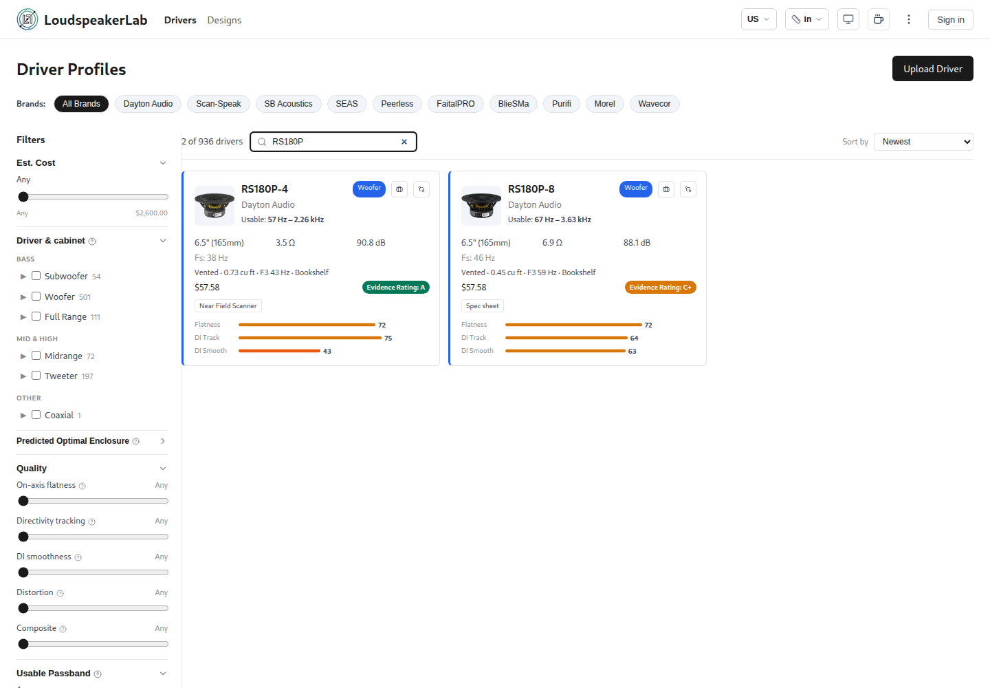
Select Add to compare on the profiles you want to inspect, then open Compare from the queue. Driver comparison places response, impedance, directivity, distortion where available, specifications, and band scores together. Compare distortion measurements only when their drive levels and measurement conditions are compatible. For a coaxial driver, select its woofer or tweeter element as needed.
The shared catalog contains manufacturer data and contributor measurements. Uploaded measurement archives are immutable once published, preserving historical evidence cleanly. Published designs retain their pinned measurement revisions, while editable drafts adopt corrected profile revisions when you edit and save, and remixes begin from the current profile revision. When a profile is superseded, a notice alerts you so you can review the change before replacing data in a project.
3.8 Evidence Grades and Band Scores
Evidence grades summarize the source and completeness of the data. The grades run from C to A. Scanner measurements generally start with a stronger evidence basis than datasheet curves, while missing information and measurement conditions affect the final score. The driver band score considers response flatness, off-axis tracking, directivity-index smoothness, and harmonic distortion where available. It evaluates a usable frequency band. Use it to compare suitability for a particular role, not as a universal ranking of driver quality.
Import checks can flag suspicious or incomplete data. They cannot certify that a measurement is free of reflections or calibration errors. Corrected profiles can supersede older ones, and affected designs can be reviewed against the updated data. Record the acquisition conditions rather than relying on the shape of the curve alone.
3.9 Removing the Measurement Cabinet's Effects and Measurement Context
When the original baffle and enclosure are known, LoudspeakerLab can estimate their effects and remove them before applying the target cabinet. This reduces the risk of applying baffle step or box loading twice. The correction uses the recorded baffle dimensions, driver position, enclosure type, volume, and tuning. It is a model-based adjustment. It cannot remove every cabinet resonance, leak, reflection, or measurement error. Drivers with sealed rear chambers do not need the same bass-loading correction as open-backed woofers.
Measurement context also determines which target enclosures a profile can support accurately. For example, a composite cone-plus-port measurement cannot drive a coupled vented or passive-radiator model that solves the port or radiator as a separate physical aperture, and filtered or multi-driver assembly curves are refused rather than silently misapplied. When a draft pauses preparation because electrical, measurement-fixture, or physical-rear details need clarification, you can record scoped design-local assumptions with a supporting source reference on that draft without modifying the shared catalog profile.
3.10 Measurement choices for an open panel or a finished assembly
If you have data for a bare or reference-mounted driver, choose Model from driver data and describe the intended panel, cabinet, or in-wall baffle. LoudspeakerLab then estimates how that new boundary changes the response. If you measured the driver in the exact target assembly or in-wall baffle with a shared time reference and known acquisition geometry, choose the measured target route. The measured assembly already contains its panel and cabinet effects, so they must not be applied again.
For a dipole or other front/rear radiator, measure both front and rear horizontal and vertical angles through the full ±180° orbit when possible. Keep microphone radius, input level, terminal polarity, and timing consistent. A gated measurement has a lower frequency limit set by the time window. A cone near-field curve does not show far-field cancellation around an open panel. At a deep null the signal approaches the noise floor, making both magnitude and phase uncertain.
With only front data, a modeled rear is an estimate. LoudspeakerLab uses tiered rear estimates ranging from a symmetric dipole baseline to a chassis high-frequency roll-off and panel-edge scaling with basket-leakage spread checks, as detailed in Section 5.11. Even with those checks, an estimated rear is not a measured description of that particular driver. Check the result's stated limits before relying on rear angles or sound power.
3.11 Upload measurements
Open Upload Driver and identify the model and measurement profile. The form can prefill shared physical specifications from canonical models or manufacturer catalog defaults, parse pasted specification-sheet text, and import measurement-fixture dimensions from a saved source. A normal upload needs an on-axis response file and an impedance file (up to 3 MiB per file in multi-file upload sessions), plus horizontal and vertical response files when you have them. The filename detector can suggest an axis and angle, and a coaxial profile keeps separate woofer and tweeter metadata and measurements so open-back woofer defaults never leak onto a sealed coaxial tweeter.
Record the driver's rear construction as open or sealed, using the automatic rule-based suggestion or overriding it manually when needed. Open-backed drivers measured inside a sealed test box remain physically open so they can load new enclosures later. Record the measurement baffle, back loading, measurement type, SPL calibration, any known acoustic-center value, and trusted T/S parameters. Context checks verify that near-field files accompany gated in-box measurements rather than scanner, already-merged, or datasheet uploads, and that port near-field files pair with cone near-field data, vented loading, cone area, and port diameter without conflicting with pre-merged port output. Consistency checks screen uploaded curves before publication.
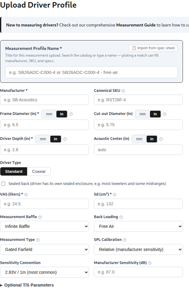
Use the edit or corrected-revision flow to update a profile you own. Upload measurements that you own or have permission to share. A driver profile is shared catalog data, while an unpublished design is a private draft. Existing designs can retain a superseded profile until their owner reviews and accepts the correction.
4. Enclosure Design
LoudspeakerLab models sealed, vented, and passive-radiator enclosures, and also lets you select pre-built cabinets from the accessories catalog. When you choose a pre-built cabinet, its exterior shape, dimensions, and panel thickness stay locked until you choose to switch to a custom cabinet. Choose an alignment that suits the driver and the space available for the build. Compare bass extension with cone excursion before settling on the volume, and use the fast Box Review acoustic tabs (Cabinet Effect, Directivity, and 3D Field) to preview baffle and radiation behavior while laying out the box.
When grouping drivers into enclosures automatically, LoudspeakerLab picks vented alignments for drivers with $Q_{ts} \le 0.6$ (when $Q_{es}$ and $Q_{ms}$ are known) and sealed alignments otherwise, never selecting a passive radiator automatically. Only the lowest-frequency bass group receives a vent automatically. Physically sealed-back drivers such as tweeters and sealed midranges stay excluded from shared internal chamber air while keeping their exterior piston radiation.
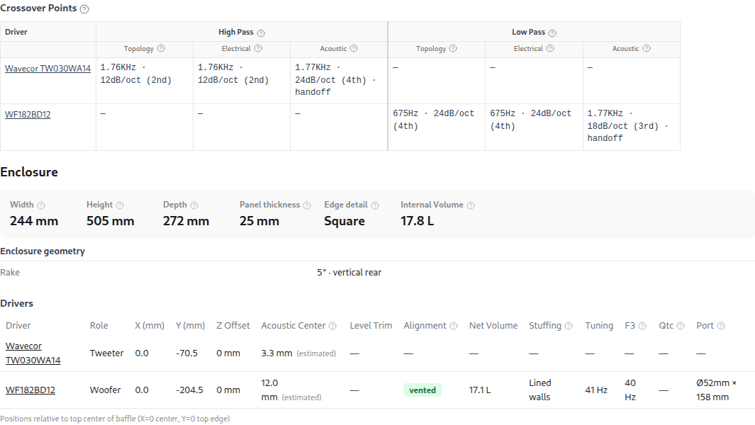
In Box Review, Auto lets the sizing calculation adjust a dimension. Fixed holds the dimension you entered. Changing volume can adjust the remaining dimensions. Review the resulting net volume and physical clearances after each change. The bass charts use the selected drive level, so compare excursion and port speed at the same level.
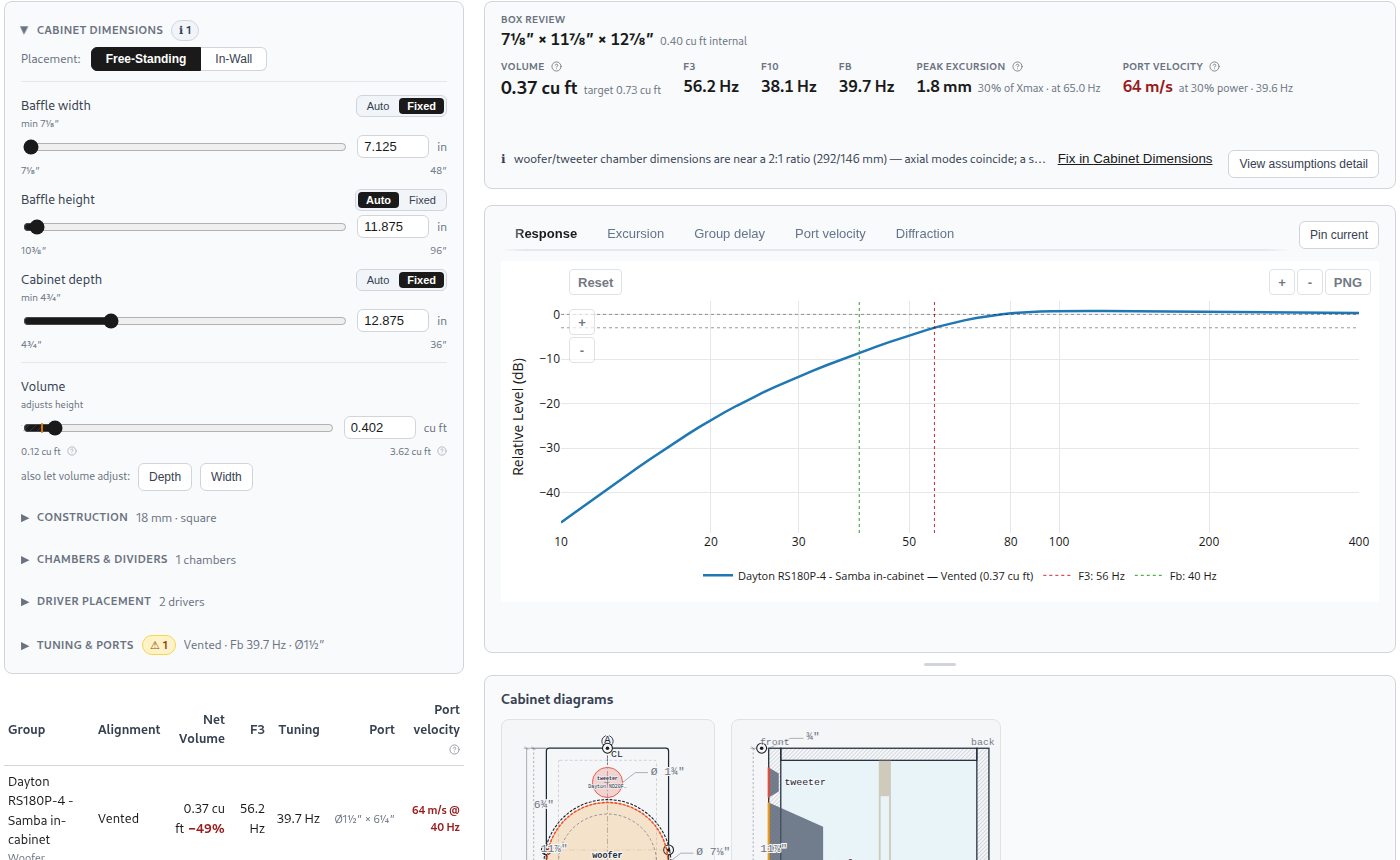
4.1 Sealed Enclosures
A sealed box adds stiffness to the driver's suspension. The ratio of equivalent compliance volume $V_{as}$ to box volume $V_b$ sets the change in the ideal small-signal model. It raises the resonance to $f_c$ and changes the system quality factor to $Q_{tc}$. The equations below omit extra box losses, which are separate assumptions in the completed design.
The low-frequency response approaches a 12 dB-per-octave rolloff. A smaller box generally raises resonance and $Q_{tc}$. Review the predicted curve rather than choosing volume from a target $Q_{tc}$ alone. Check excursion at the intended drive level as well as the bass extension.
4.2 Vented Enclosures
A vented box couples the air mass in its port with the compliance of the enclosed air. Its volume, port area, and effective length determine the tuning frequency. The port contributes output near tuning while reducing the cone motion needed there. Below tuning, that benefit falls away and cone excursion becomes an important design limit.
The alignment choices include B4, QB3, and SBB4. Their suggested volume and tuning depend on the driver's parameters. The response approaches a 24 dB-per-octave rolloff at sufficiently low frequencies, and cone excursion can become excessive below tuning. A high-pass below the useful band can be part of an active design when sub-tuning excursion needs control.
4.3 Ports and Air Velocity
The port calculation includes the duct, the opening through the panel, and an end correction. Box Review supports one to three round ports (on the back, bottom, or front baffle, arranged vertically or horizontally when using multiple non-bottom ports) as well as front slot ports. Physical limits require at least a 20 mm diameter for round ports and at least a 12.7 mm height and 30 mm length for front slot ports, and impossible cabinet volumes or port geometries are blocked before saving. Increasing port area reduces air velocity for a given volume flow, but it also requires a longer port at the same volume and tuning. Check that the duct fits inside the cabinet and that its internal opening is not obstructed. Use the displayed port controls to hold dimensions or tuning fixed while the remaining value is calculated.
Velocity warnings use practical thresholds of 20 m/s and 28 m/s. These are design checks, not a calculation of turbulence or a guarantee of inaudible port noise. Actual noise depends on the port shape, flares, signal, and level. A very high predicted velocity indicates that the small-signal model is being used beyond a credible operating range.
4.4 Passive Radiators
A passive radiator replaces the port's moving air mass with an unpowered diaphragm. Added mass changes the tuning. Its suspension and internal enclosure losses affect the response, so it should not be treated as an ideal port at every frequency. The available travel and added mass also need to suit the chosen physical radiator.
In Box Review, you can select one to four matching catalog passive radiators mounted on the baffle or back, set added mass automatically or to a fixed value, and inspect the notch frequency readout. Box Review plots the active driver's cone excursion and flags a low-displacement warning when combined radiator displacement falls below the driver's volume displacement, rather than plotting passive-radiator travel versus frequency directly. During full-wave cabinet preparation, however, the coupled acoustic model solves the passive radiator's diaphragm motion and separate exterior radiation directly as its own physical aperture.
4.5 Fill and Losses
Cabinet fill is represented by an increase in effective acoustic volume. The current factors are 1.00 for bare walls, 1.05 for lined walls, 1.12 for half fill, and 1.20 for full fill. These are empirical assumptions. The result depends on the material and how it is installed. Leakage and absorption are represented by loss factors. Review the assumptions attached to the design, particularly when comparing modeled results with a physical cabinet.
4.6 Cabinet Dimensions and Internal Space
Net acoustic volume excludes the estimated space occupied by drivers, ports, dividers, and bracing. Exterior box limits extend up to 1,219 mm (48 in) wide, 2,438 mm (96 in) tall, and 914 mm (36 in) deep, with a default panel thickness of 18 mm. For multi-region builds, the Chambers and Dividers construction editor lets you define closed versus open regions, dividers, sub-enclosures, window braces, ports, passive radiators, and supports. Check the final internal dimensions after changing any of these values. Dimension warnings identify nearly equal dimensions and simple ratios that can place axial resonances close together. This is a proportion check. It does not predict the complete internal sound field or cabinet-panel vibration.
4.7 Cabinet Views, Finishes, Build Sheets, and AR
Cabinet options include five shapes: rectangular, tapered-shoulder, arched-top, stepped-baffle, and stacked-module layouts. Front rake from 0° to 20° and rear wall options (vertical, parallel, or opposed) act as modifiers across those shapes, including per-module rake on stacked towers. Tilting the baffle with rake changes the vertical listening axis relative to the cabinet without double-counting driver depth offsets or inter-driver time delay. Placement can also be set to Free-Standing or In-Wall, and the drawings and 3D view help inspect driver placement, proportions, ports, and edge treatments.
The finished 3D view supports uniform or per-face and per-module wood and paint finishes with baked ambient occlusion, and saving a published design freezes its chosen finish. You can rotate the 3D view, return to the front view, or reduce cabinet opacity to inspect the interior. Driver models may be generic, as the viewer indicates. The 3D view helps check appearance and layout, but it is not a manufacturer-certified mechanical drawing.
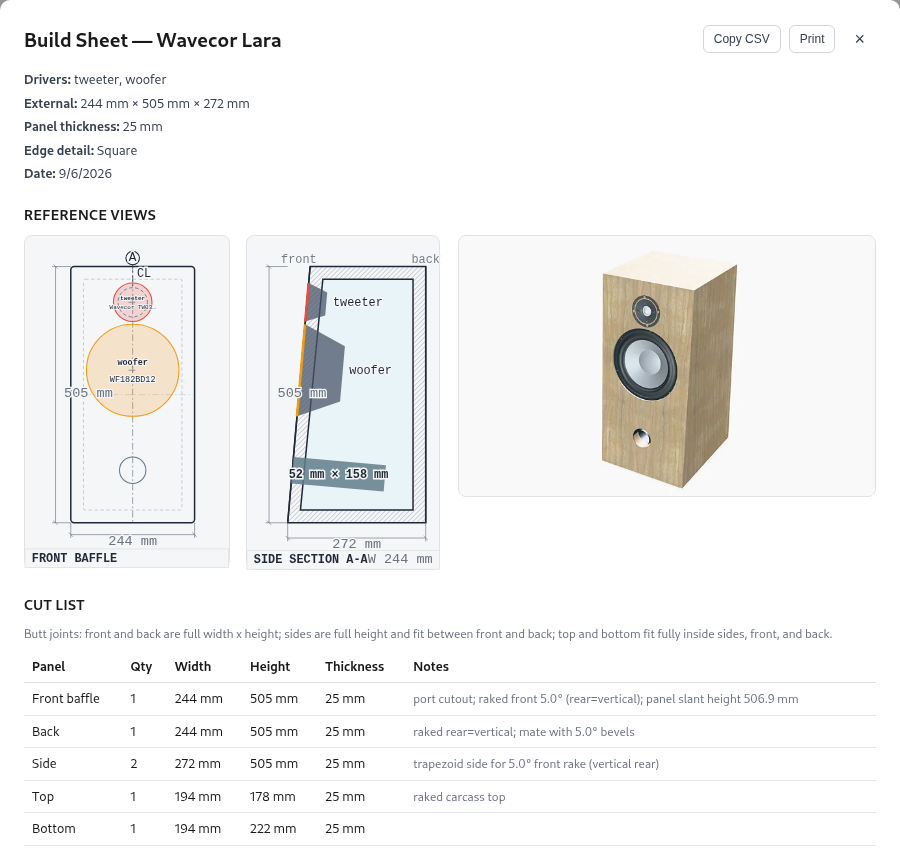
The build sheet provides panel dimensions, cutout positions, and a sheet-layout estimate with kerf and trim allowances. Check the actual driver, port hardware, joint details, and material thickness before cutting. Commercial flat-pack options also need a final fit check. On supported mobile devices, the viewer can open an augmented-reality placement view through the available WebXR, Quick Look, or Scene Viewer integration. AR shows approximate size and placement in the camera view. It does not predict room acoustics or replace physical clearance measurements.
4.8 The transfer functions behind the bass curves
A transfer function gives the response at each frequency relative to a reference input. In the ideal sealed-box model from Section 4.1, let $s=j2\pi f$ and $\omega_c=2\pi f_c$. The response is given by the following equation. Using the same reference is essential when comparing the driver alone with its loaded response.
The displayed $F_3$ is the frequency 3 dB below the selected reference level. It need not equal the box resonance $f_c$. A vented box couples the moving cone to the air in its port. With $u=jf/f_s$, $h=f_b/f_s$, $Q_L$ the combined loss factor, and $\alpha=V_{as}/V_b$, the following equation gives the normalized response.
A passive radiator has its own moving mass $M_{PR}$ and compliance $C_{PR}$. Its free resonance is $F_{PR}=1/(2\pi\sqrt{M_{PR}C_{PR}})$. Added mass lowers this resonance. The available volume displacement is $V_d=S_dX_{\max}$, where $S_d$ is effective diaphragm area and $X_{\max}$ is the stated linear travel.
The sealed-box analysis by Small sets out the compliance and damping relationships used here. Thiele and Small describe the coupled vented-box response and its losses. Small’s passive-radiator analysis includes the unpowered diaphragm’s own mass and suspension. These are small-signal models, so their predicted response does not establish high-level compression or turbulent port behavior.
4.9 What the geometry model accepts
The drawings and 3D viewer can show more layouts than the detailed full-wave acoustic solvers accept, so check these boundaries before relying on a prepared radiation model. For closed cabinets, full-wave boundary and coupled chamber calculations accept rectangular, tapered-shoulder, arched-top, and stepped-baffle cabinets, stacked multi-module assemblies of two to five rectangular or raked modules, front and rear rake, chamfered and rounded edges on ordinary and stepped cabinets, recessed driver pockets on closed boxes and modular stacks, rear, side, top, and bottom driver mounts on ordinary boxes and pure closed constructions, shared air chambers (such as dual-woofer or woofer-tweeter-woofer layouts), round vented ports, equal-area front slot port estimates, passive-radiator chambers, and closed-cabinet dipole or bipole driver pairs.
Several combinations are refused or restricted by the detailed physics models. Stepped baffles, stacked modules, and open panels accept front-mounted drivers only, and stepped baffles cannot place a port on the stepped front baffle. Stacked modular towers require square edges, two to five non-overlapping modules, and chambers that do not span across separate modules. Back-wall ports and passive radiators require a vertical rear wall, and side, top, or bottom ports and passive radiators are not accepted by the full-wave chamber model. Recessed driver pockets are refused on open panels and hybrid panel-over-box constructions, while hybrid panel-over-box designs require open regions above the closed box without rake, tapered, arched, or stepped shapes. Concave seams and faceted curved surfaces also carry explicit coverage caveats in the saved design assumptions. A finish changes the appearance of the cabinet only, and AR placement inspects size without modeling room reflections.
5. Cabinet effects and directional radiation
A loudspeaker cabinet or panel is a full 3D acoustic boundary that reshapes radiation, impedance, and off-axis balance well beyond a simple flat-baffle step. For all new supported closed cabinets, stacked towers, open panels, and hybrid panel-over-box builds, LoudspeakerLab computes 3D Boundary Element Method (BEM) radiation at low and mid frequencies blended smoothly into Svensson finite-edge diffraction at high frequencies, coupled with internal chamber, port, and passive-radiator loading. This chapter explains how to read those full-wave Cabinet Effect views and how the BEM, edge-diffraction, and coupled-chamber models operate.
5.0 Read the Cabinet Effect view
The Cabinet Effect tab presents the prepared full-wave Radiation Atlas for your loudspeaker. You can inspect horizontal and vertical contours across the full ±180° orbit, explore an interactive 3D radiation globe, read complex level and phase spectra in any direction, compare against each driver's loaded response before cabinet radiation, and check model labels and provenance indicators. Older published designs saved before full-wave modeling (or narrow fallback cases lacking required physical parameters) display their legacy scalar front-baffle curve over the front ±90° hemisphere instead.
Viewing Cabinet Effect always reads pre-calculated baked results and never triggers a slow surface calculation just by opening the tab. When you modify a cabinet or panel construction, an inline progress bar reports background preparation status while you keep working or wait for the updated fields to finish.
In a prepared view, choose the source and its horizontal and vertical angles. On-axis returns both angles to zero. Listening axis chooses the nearest prepared angles to the current listening direction. Hover over the direction spectrum to read its level and phase at a frequency. Show phase adds a phase plot.
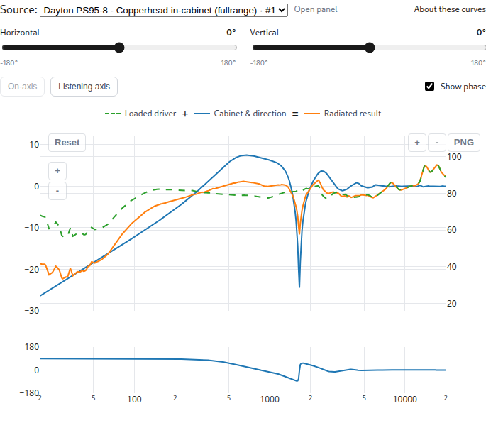
The dashed green Loaded driver curve is the on-axis driver after its air or box loading, before the cabinet and crossover. The blue Cabinet & direction curve shows the change caused by the cabinet and the chosen direction. It uses the left dB scale. The orange Radiated result uses the right SPL scale, as does the green curve. At each frequency, the green SPL plus the blue change gives the orange SPL. Hover over the line names for their definitions.
The BEM band shows the complete cabinet effect because its interacting wave contributions cannot be separated into independent corrections. Coverage labels and hover details identify accepted frequencies and directions. Unavailable values are hidden. A deep null can make phase unreliable.
A loaded-source reference compares radiated pressure with that driver’s on-axis response after its air or box loading but before its cabinet effect. The on-axis row therefore shows cabinet gain, which need not be 0 dB. In the contour controls, Actual SPL shows the prepared source level. On-axis relative compares each direction with the source’s radiated on-axis response. Loaded-source relative compares it with the loaded driver before cabinet radiation.
Both references are complex pressures. Dividing them preserves the phase relationship. Subtracting two separately wrapped phase angles can give the wrong result. A near-zero reference or response is masked because its phase is not useful.
Horizontal Contour and Vertical Contour initially show the system after the crossover. Where prepared data are available to the owner, the source selector can show an individual driver. Front ±90° and Full ±180° crop the viewport without recalculating the model. A front-only dataset remains front-only. The full view is especially useful for an open baffle or closed-body 3D field because it includes the rear lobe.
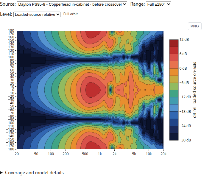
The normalized horizontal and vertical views share a range from −30 to +12 dB. This keeps a rear lobe stronger than the reference axis visible. Inspect in 3D opens the same cabinet scene used by Show environment. The display reads prepared results, so opening it does not start another surface solve.
5.1 Full-Wave BEM and Edge-Diffraction Cabinet Radiation
LoudspeakerLab models the exterior acoustic field directly from the 3D geometry of your enclosure or panel. Below a geometry-dependent split frequency ($f_{\rm split}$), the cabinet or panel surface is discretized into a triangular mesh and solved via the Galerkin Boundary Element Method (BEM). Closed cabinets use the Burton–Miller boundary integral formulation to eliminate fictitious interior resonance errors, while open panels use a slab BEM formulation across both faces. This solves low-frequency baffle step, cabinet depth, edge wrap-around, mutual radiation impedance, and rear radiation straight from the 3D shape.
Above $f_{\rm split}$, where wavelengths become much smaller than the cabinet, LoudspeakerLab transitions smoothly across a one-third-octave band in complex pressure to first- and second-order Svensson finite-edge diffraction over the 3D edges of the cabinet or panel. Both bands are driven by each driver's own measured infinite-baffle response (with known measurement-fixture effects removed once), preserving measured cone breakup and directivity across the full $\pm 180^\circ$ horizontal and vertical radiation spheres.
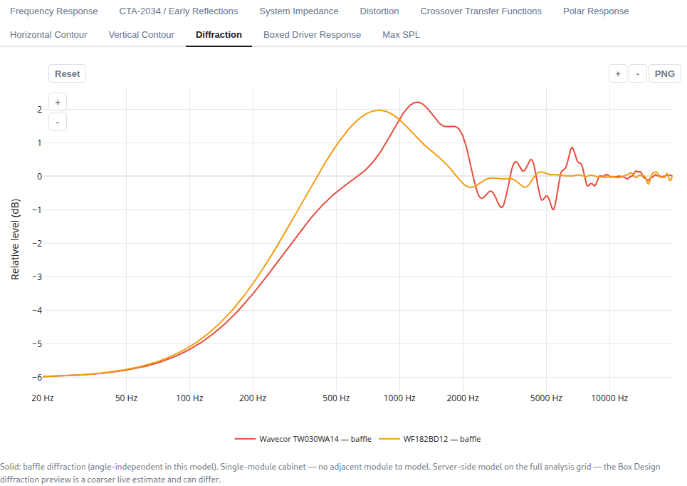
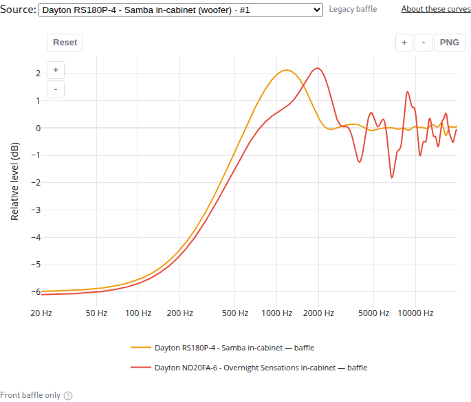
For backward compatibility, older designs pinned before full-wave modeling (as well as narrow fallback cases where full-wave chamber data are unavailable, such as vented cabinets missing motor parameters) retain a scalar front-baffle impulse estimate informed by Vanderkooy's cabinet-edge theory and clearly labeled in Cabinet Effect. The two historical figures below illustrate those legacy front-baffle views from earlier saved designs.
5.2 Coupled Chamber Loading and Live Box Review Previews
For closed cabinets with vented ports, passive radiators, or shared internal air chambers (such as dual-woofer or woofer-tweeter-woofer layouts), LoudspeakerLab solves a coupled mechanical-electrical-acoustic system across all chamber apertures by default. This combines exterior self and mutual BEM radiation impedance, uniform interior cavity compliance and losses (valid below the first axial cabinet mode), and reflected electrical impedance seen by the crossover. Ports and passive radiators radiate through their own separate exterior 3D BEM and edge fields at their realized physical cabinet locations rather than being lumped onto a woofer axis.
Because preparing a full 3D BEM mesh and surface solve takes tens of seconds to a few minutes, interactive editing inside Box Review uses a fast 81-point (one-eighth-octave, 20 Hz to 20.48 kHz) perimeter diffraction preview across its Cabinet Effect, Directivity, and 3D Field tabs. Use that quick preview to explore driver placement and box proportions, then allow full-wave BEM preparation to complete when saving the cabinet or construction.
5.3 Radiator Size, Placement, and Recessed Pockets
In the BEM and edge-diffraction pipeline, each driver's effective piston radius $a$ defines the moving surface patch on the 3D mesh and determines its self and mutual radiation impedance. Offsetting a driver laterally or vertically separates edge-path lengths across the 3D boundary, reducing symmetric interference ripples in both the BEM and Svensson edge bands.
To prevent ideal rigid-piston nulls from being falsely imprinted onto real cones at short wavelengths, LoudspeakerLab blends smoothly between $ka = 2.5$ and $ka = 3.8$ toward the driver's measured direct response combined with 3D edge diffraction. When a driver sits in a flush-recessed pocket on a supported closed box or stacked module, a local infinite-baffle pocket diffraction factor models the pocket lip alongside the flush BEM surface mouth.
5.4 Cabinet Shapes, Edge Treatments, and Rake
Unlike flat-baffle diffraction calculators, the full-wave BEM and edge-diffraction model operates on true 3D cabinet geometry. Supported rectangular, tapered-shoulder, arched-top (realized as a faceted convex polyhedron), and stepped-baffle profiles, along with front rake (0° to 20°), rear wall orientation (vertical, parallel, or opposed), chamfered edges, and rounded edges (faceted BEM mesh paired with tangent-chamfer high-frequency edges), directly shape the 3D acoustic boundary. Because curved facets and rounded transitions are discretized cleanly within the solver's rules, inspect the coverage notes in your design assumptions when comparing subtle edge treatments.
5.5 Stacked Modules
Prepared stacked multi-module towers of two to five separated or face-contacting rectangular or raked modules are solved together as one coupled exterior 3D BEM and edge-diffraction assembly. Inter-module steps, overhangs, and front-baffle reflections arise naturally from the combined 3D surface rather than an approximate mirror-source add-on. Check the saved design's assumptions to inspect coverage boundaries across complex multi-module seams.
5.6 Open baffles, dipoles, bipoles, and cardioids
A radiation pattern describes where a speaker sends sound, while a cabinet type describes what surrounds the cone. An open-backed cone produces front and rear radiation, and a pair of boxed drivers mounted front and back on a closed cabinet can also form a directional pattern modeled directly by the closed-body BEM and coupled-chamber solvers. Wiring polarity, source spacing, and filtering all affect that pair. Choose the physical construction first and inspect the calculated pressure pattern before relying on a dipole, bipole, or cardioid label.
| Arrangement | What moves and radiates | Expected low-frequency behavior |
|---|---|---|
| Conventional closed cabinet | The cone radiates outside. Its rear works against enclosed air. | Roughly omnidirectional when the cabinet is small compared with a wavelength. |
| Open baffle | One cone radiates from both sides of a finite panel. | Front and rear pressure have opposite signs. They cancel at the sides and partly cancel in front at low frequencies. |
| Dipole pair | Two separate, oppositely facing drivers have opposite acoustic polarity. | A figure-eight pattern in the compact-source limit. Each driver still has its own load and filter. |
| Bipole pair | Two oppositely facing drivers have the same acoustic polarity. | Their bass adds. The pair approaches an omnidirectional source when its spacing is small compared with a wavelength. |
| Cardioid or endfire arrangement | Separate sources use a chosen mixture of level, polarity, spacing, and delay. | Cancellation can favor one direction. The shape changes with frequency and real driver behavior. |
One open-backed cone is one electrical load, even though it radiates from both faces. It therefore needs one branch in the crossover. A front/rear pair has two physical drivers with their own electrical loads, mounting, and loading. Its rear source cannot be represented by duplicating the front curve without accounting for that second driver.
The current pair presets require matching driver identities, opposing mounts, and separate sealed chambers. Bipole sets relative branch wiring polarity to +1. Dipole sets it to −1. If mounting, loading, or wiring no longer matches the preset, the arrangement becomes Custom. A label alone never replaces the pressure calculation. General U-frame, H-frame, horn, and arbitrary shared-chamber models are not implied by these presets.
Read the equations for panels, diffraction, loading, and directional pairs
5.7 Why a dipole loses bass: a useful first calculation
Let $f$ be frequency in hertz, $c=343$ m/s the sound speed, $\lambda=c/f$ wavelength, and $k=2\pi f/c$ wavenumber. Let $d$ be the spacing of two ideal point sources and $\theta$ the angle from their front-to-back axis. With time convention $e^{j\omega t}$, a traveling wave has phase $e^{-jkr}$. These definitions let you compare the source spacing with wavelength before considering a particular driver or cabinet.
After removing a common distance factor, equal sources at $z=+d/2$ and $z=-d/2$ give:
The plus sign describes an ideal bipole. The minus sign describes an ideal dipole. Both results depend on source spacing relative to wavelength. When $kd\ll1$, $P_-\approx jkd\cos\theta$. Three results follow:
- Halving frequency halves pressure: $20\log_{10}(2)=6.02$ dB less output per octave, relative to the same sources without cancellation.
- At $90^\circ$, $\cos\theta=0$: an ideal dipole has a side null.
- Front and rear have equal magnitude but opposite phase. A graph of magnitude alone hides this difference.
For example, $d=0.20$ m at 50 Hz gives $kd\approx0.183$. The front magnitude is about 0.183 relative to one unit source, or −14.8 dB. This illustrates cancellation. It is not a prediction for a 20 cm wide panel. The path around a real panel depends on its whole outline, cone position, thickness, and frequency. LoudspeakerLab uses the panel calculation below instead of fitting a single effective spacing.
An ideal normalized dipole has $D(\theta)=\cos\theta$. Its sphere-average squared pressure is $1/3$, giving directivity factor 3 and directivity index $10\log_{10}(3)=4.77$ dB. An ideal cardioid $D=(1+\cos\theta)/2$ has the same factor but a rear null instead of two equal lobes. These are useful checks, not universal values for real speakers.
For independently driven sources, replace their unit strengths with complex weights $w_F(f)$ and $w_R(f)$:
In this ideal example, choosing $w_F=1$ and $w_R=-e^{-jkd}$ cancels the rear direction. It means invert the rear source and delay it by $d/c$. In the compact limit the remaining pattern is proportional to $1+\cos\theta$, but forward output also falls toward zero as frequency falls. Real cabinet diffraction and unequal drivers change the required weights. This explains cardioid/endfire theory. It does not establish a validated automatic cardioid optimizer or broadband hardware result.
5.8 The finite-panel calculation at low frequencies
The open-panel model treats the panel as rigid and the cone as a circular piston. It solves the air outside the panel. It does not simulate panel flexing, a room, or turbulent flow. The cone’s prescribed motion is the source that drives the surrounding air.
Pressure obeys the Helmholtz wave equation:
Here $\nabla^2$ measures how pressure curves through space, $\rho_0$ is air density, and $v_n$ is surface velocity pointing out into the air. On the rigid panel $v_n=0$. On the front piston it is $+v$. On the rear it is $-v$. This is one moving cone, not two independently powered sources.
The boundary element method (BEM) breaks the panel surface into small triangles. It finds the pressure on those triangles and then calculates the sound radiated into the surrounding air. The mesh represents the panel outline, its thickness, and the moving piston area. The expression below gives the wave contribution at point $x$ from point $y$, including its phase and distance dependence.
The panel uses the following boundary equation.
$I$ is the identity operator, $K'$ describes one surface-to-surface interaction, and $W$ describes the normal-derivative interaction. Its integrated form is
The subscript $S$ means changes along the surface. The test function $\psi$ asks whether the computed pressure satisfies the equation over a small patch. Both pressure and test functions vary linearly over each triangle: this is a P1 Galerkin method. The result is a complex matrix equation, solved separately at selected frequencies.
The two sides of a panel have opposite source motion. That symmetry reduces the number of unknown pressures. A centered driver can also use left/right symmetry. The interaction between nearby triangles is difficult because $G$ grows as their separation $R$ approaches zero. The calculation separates its static $1/(4\pi R)$ term, integrates nearby interactions semi-analytically, and uses numerical quadrature for the smooth remainder.
The calculation uses several mesh resolutions across frequency bands. It solves sparse frequency knots, then interpolates complex pressure, preserving cancellation and phase. This is a numerical approximation to the stated boundary problem. Mesh convergence and independent references determine its accuracy.
5.9 Edge diffraction at high frequencies
At short wavelengths, a full surface solve becomes expensive. The panel calculation uses first- and second-order Svensson edge diffraction. First order follows a path from source to edge to listener. Second order passes over two edges. Visible direct sound and edge sound are added as complex pressure.
For a finite edge, the first-order correction relative to a direct path of length $r$ is
$m$ is source-to-edge distance, $\ell$ edge-to-listener distance, and $z$ position along the edge. These distances set the phase delay of each edge path. For material wedge angle $\gamma$, $\nu=\pi/(2\pi-\gamma)$. A square slab edge has $\gamma=\pi/2$. The angular factor is
The angles and radial distances here are measured around the edge, not around the speaker axis. Illuminated edge intervals are integrated with eight-point Gauss–Legendre quadrature. At shadow boundaries it combines the special edge limit with half-weight geometric sound. Second order integrates over visible edge pairs. Far-field plots use the analytic infinite-distance limit of the kernel, not a microphone placed at an arbitrary large distance.
For smaller panel extent $L$ and thickness $t$, the panel's switch frequency is
The thickness bound is omitted for an infinitely thin panel. The first bound is about 3.5 wavelengths across the smaller panel dimension. The switch therefore depends on the physical dimensions of the panel. Across the final one-third octave below this frequency, the models blend in complex pressure.
Outside that interval, $w$ is 1 below it and 0 above it. The high-frequency estimate includes second-order edge paths through 6 kHz. It treats the outer edge of an arched panel as a rectangular bound, so the predicted high-frequency diffraction of that curve is approximate. Above the blend, the edge model supplies the panel field used in the response.
5.10 Combining the panel with real driver measurements
A perfect piston does not include a real driver's breakup peaks or directivity. LoudspeakerLab therefore starts with that driver's own infinite-baffle response, after removing a known measurement box and baffle once. The panel correction changes how that measured source radiates in its new surroundings. Its measured response shape remains the source basis for the calculation.
Let $H$ be the driver's complex response in the facing direction, $g$ its on-axis response, $H_g$ its response at grazing incidence (90°), $T$ the ideal-piston panel field, and $D$ the ideal piston directivity:
$a$ is piston radius and $J_1$ is a Bessel function. In the BEM band the measured response becomes
$D_{\rm reg}$ preserves the sign of $D$ but has magnitude at least 0.25. Away from a piston null this reduces to $HT/D$. Near a null it prevents division by nearly zero. If the driver is exactly a piston ($H=gD$), the answer remains exactly $gT$. At higher frequencies where cone breakup departs from rigid-piston behavior (transitioning smoothly between $ka = 2.5$ and $ka = 3.8$ when the mounting face is large enough relative to wavelength), the factorization blends toward measured direct sound plus edge contributions so ideal-piston nulls are not falsely imprinted onto real cones.
In the edge band, the measured direct sound is added to edges excited by $H_g$. The front and rear faces each contribute their own visibility, position phase, and source sign. This matters because an edge hears the cone nearly sideways. Using the on-axis response for all edges would overstate high-frequency edge excitation.
Combined horizontal and vertical angles use stored panel fields:
$Q$, $P_g$, and $P_h$ are geometry-dependent complex coefficients. $h_f$ is the angle seen from the facing hemisphere. This $Q$ is a field coefficient, not a resonance quality factor. The field grids use 10° steps below 500 Hz and 5° above. This replaces ordinary separable H×V lookup for these modeled sources: multiplying two dipole plane cuts would give the wrong diagonal pattern. Symmetrically centered layouts enforce exact bilateral horizontal symmetry, continuous vertical meridian unfolding avoids artificial rear-hemisphere contour discontinuities, and null-safe complex lookup prevents inventing phase where pressure vanishes.
5.11 Estimating a missing rear response
Front measurements do not reveal how a basket and magnet obstruct rear sound. When rear measurements are unavailable, LoudspeakerLab provides tiered estimation checks rather than claiming measured hardware behavior. A real rear measurement carries that hardware behavior into the source data, whereas an estimated rear remains an explicit design assumption.
The baseline symmetric dipole drives the rear with opposite sign at unit strength. An optional chassis roll-off reduces and delays high-frequency rear drive above $f_{\rm compact}$ using the following relationship:
The corner $f_c$ can be declared explicitly. Below the compact threshold $s=1$, and at higher frequencies it attenuates and delays the rear excitation. LoudspeakerLab also supports an edge-ratio tier above $f_{\rm compact}$ derived from the panel's high-frequency outline and a basket-leakage spread check across driver families. Unless the third-octave spread of that rear estimate stays within 6 dB, dipole or cardioid CTA-2034 sound-power and directivity-index authority is withheld.
The BEM source is assembled with the following relationship.
The odd field is the dipole. The even field uses the thin-slab breathing approximation. At $s=1$ this is the symmetric dipole. At $s=0$ it is a front-only source. In the edge band the same $s$ multiplies the rear face's entire direct-plus-edge contribution. Changing rear drive therefore changes front diffraction and sound power too, not just the rear graph.
This selection is limited to modeled open panels. It cannot turn a physically sealed-back driver into an open-backed cone, and it is refused on sealed-back drivers unless test-box front measurements are explicitly declared. Source loading still assumes the symmetric piston, and no driver-specific accuracy band is claimed for any rear estimate.
5.12 The panel also changes cone motion and impedance
Air pushes back on the cone. Its radiation impedance is force divided by velocity, measured in N·s/m. Changing the surrounding panel changes that load, so changing only the SPL curve would leave the electrical and excursion predictions inconsistent. That coupling is included before crossover filtering is evaluated.
Let $Z_p$ be the panel air load, $Z_{IB}$ the two-face infinite-baffle load, and $Z_f$ the free-disc load. With electrical baseline $Z_e=R_e+j\omega L_e$, motor force factor $Bl$, and free-disc air mass $m_0=8\rho_0a^3/3$:
Subtracting $m_0$ avoids counting air mass twice: measured moving mass $M_{ms}$ already includes it. At equal drive voltage, the response and free-air excursion corrections are
The loaded electrical impedance is given by the following relationship.
Near a zero in a denominator, the calculation limits the correction. It also fades the impedance adjustment between $ka=1$ and $ka=2$ to preserve the measured high-frequency behavior. Loading needs sufficient T/S data. Mutual air loading between separate cones on a pure open panel is not included. Acoustic pressure summation alone does not solve that feedback.
Boosting deep bass can restore a plotted level but consumes excursion and amplifier voltage. An extra 6 dB requires about twice the voltage and cone motion in the linear model. This is why an open-baffle design needs output-limit checks as well as a flat response. A steeper low-frequency high-pass can reduce that demand by restricting the band the driver is asked to cover.
5.13 Closed cabinets, coupled chambers, and mixed open/closed constructions
Closed cabinets, stacked towers, and open-panel-over-box hybrids use the closed-body BEM solver below $f_{\rm split}$ and Svensson finite-edge diffraction on the union of convex blocks above, while an open panel over a closed bass box combines the panel and body formulations. Choose geometries within the accepted construction rules in Section 4.9 so every boundary and chamber aperture resolves cleanly.
A closed surface has mathematical interior resonances that can spoil a single boundary equation. The Burton–Miller method combines two equations to remove that ambiguity:
$M$ is the surface mass matrix, $S$ and $K$ are the single- and double-layer interaction matrices, and $b_W$ is the prescribed-velocity right side of the equation. Where chambers share air across multiple cones or drive round ports or passive radiators, LoudspeakerLab solves a frequency-by-frequency coupled mechanical-electrical-acoustic system across all chamber apertures (driven cones, undriven cones, round ports, and passive radiators).
Here $Z_m(\omega)$ combines the full exterior self and mutual BEM radiation impedance matrix (inside the BEM band) with uniform interior chamber air compliance, uniform chamber leakage and absorption losses, flanged interior cone air mass, and inner-end port tube air mass. The force-factor matrix $G$ maps branch currents $I$ to aperture forces ($Bl$ on driven cones and zero on ports or passive radiators), $Z_e(\omega)$ is the blocked voice-coil impedance (fitted from measured impedance data where available), and $v$ is the solved aperture velocity vector evaluated jointly with each branch's passive crossover network. Because ports and passive radiators act as unpowered mechanical degrees of freedom, they radiate through their own separate exterior cabinet fields at their actual realized positions rather than simply being lumped at a driver center.
The coupled chamber model operates within explicit physical bounds. The uniform-pressure interior cavity model is valid below the first axial cabinet mode $f_1 = c/(2 L_{\max})$, and higher-order interior chamber standing-wave modes plus spatially resolved wall absorption are not enabled in production. Front slot ports use an equal-area circular front-baffle estimate, and recessed pockets use a local infinite-baffle pocket diffraction factor while the surface mesh resolves the flush mouth. Coupled chamber solving also requires cone-only measurements (rather than pre-merged cone-plus-port files) and independent per-branch wiring for coupled chambers. Stacked towers of two to five modules solve exterior radiation as a single scene, while concave panel-over-box seams, second-bounce reflection-to-edge interactions, and faceted curved surfaces carry explicit acceptance caveats.
A sealed-back source's off-plane rear field above 1.5 kHz is marked interpolated rather than pointwise accepted because rear diffraction varies more quickly in angle than the stored field grid. Hybrid open sources also carry a rear high-frequency limit above their split where the edge model lacks some inter-block paths. Good averaged CTA curves do not prove accurate pressure at every rear angle, so use the marked direction and frequency limits when interpreting a source spectrum or balloon.
5.14 Measured assemblies, sound power, and validation
There are two distinct input routes. Model from driver data removes known measurement conditions and applies the chosen panel, cabinet, or in-wall boundary once. Measured in the target assembly retains that assembly's complex pressure and bypasses a second radiation correction. It requires the declared geometry and acquisition setup to match, and in-wall placements use half-space or target-measured assumptions accordingly. Moving a driver to another cabinet invalidates a target-measured claim.
Full-space measurements should cover signed horizontal and vertical orbits through ±180°, with common timing, terminal polarity, level, and radius. A magnitude-only curve or minimum-phase reconstruction cannot recover a measured dipole's front/rear timing. A cone nearfield measurement is not the far-field result of front/rear cancellation. Near nulls, phase becomes noise-sensitive because the sound itself is very small.
The physical sound-power average is proportional to the following integral.
LoudspeakerLab estimates sound power from its CTA-2034 horizontal and vertical angle samples. Open-panel and closed-body results use full front and rear orbits so the rear lobe contributes. Sound energy is averaged across different directions after the drivers' pressures have been added within each direction. Front-only measurements miss rear energy. Filling a sphere by multiplying two measured plane cuts can also misrepresent an open panel. Directivity index compares listening-window level with sound-power level.
The panel calculation has been checked against an exact solution for a circular screen and independent numerical calculations for flat and arched panels. These checks support the method for the tested shapes. They do not establish accuracy for every driver, an unmeasured rear response, or unsupported geometry. Check the limits stated with each design.
Preparing a new panel calculation can take tens of seconds, and a closed-body calculation can take minutes. A cabinet change can therefore take longer than a crossover edit. Wait for the completed result before using its plots. Returning to an unchanged prepared cabinet reuses its cached baked calculation.
5.15 Choosing and checking a directional design
The Box Review Cabinet: Box | Open baffle choice sets the boundary around the drivers. A whole open panel lets a rear-open cone radiate from both faces while retaining one electrical branch. The construction editor also describes closed and open regions, front and back mounts, and pair arrangements. A dipole pair uses opposite relative wiring polarity, while a bipole pair uses matching polarity. Those labels depend on the actual sources, mounting, and chambers rather than a duplicated response curve.
The Endfire cardioid panel applies a starting preset for accepted opposed sources on different amplifier channels. Save or discard existing crossover edits before applying it because it uses the saved geometry and channel map. Choose the front and rear sources, then select Apply endfire preset. The preset adds the relative inversion and rear delay as one undoable edit. Its status shows the requested and achieved delay and explains unavailable or stale settings. Inspect the completed front and rear response before treating it as a useful cardioid design.
A detailed panel or cabinet calculation can require background preparation. If Cabinet preparation opens, review its status and continue to the draft when it is ready. A failed preparation offers Retry preparation. Returning to the design lets you inspect the previous saved result while a new geometry is being prepared.
When evaluating an open design, inspect the entire ±180° pattern, not just the front axis. Check low-bass cancellation, side nulls, rear output, sound power, and the extra cone motion that bass equalization can demand. At a chosen listening position, the drivers' separate distances and directions affect their phase and directivity. A cardioid-like response can be designed with two controlled sources and a delay, but the guide's ideal cardioid equation is a starting point for interpretation, not a promise of automatic wide-band cardioid optimization.
The calculation is for free-field sound. In a room, rear output can reflect from the wall behind the speaker. Placement therefore matters greatly, but the plotted Predicted In-Room curve is an angular summary, not a simulation of your room. Prototype measurements remain the way to establish the result in the intended space.
6. Crossover Design
The crossover editor shows the electrical network feeding each driver, preserving each driver's branch identity, filter chain, and plot label across edits, reorders, coaxial woofer or tweeter elements, and Auto-Solve runs. Select a component to inspect its value and available properties. Response previews update immediately while you edit, and the full settled result follows shortly after you pause.
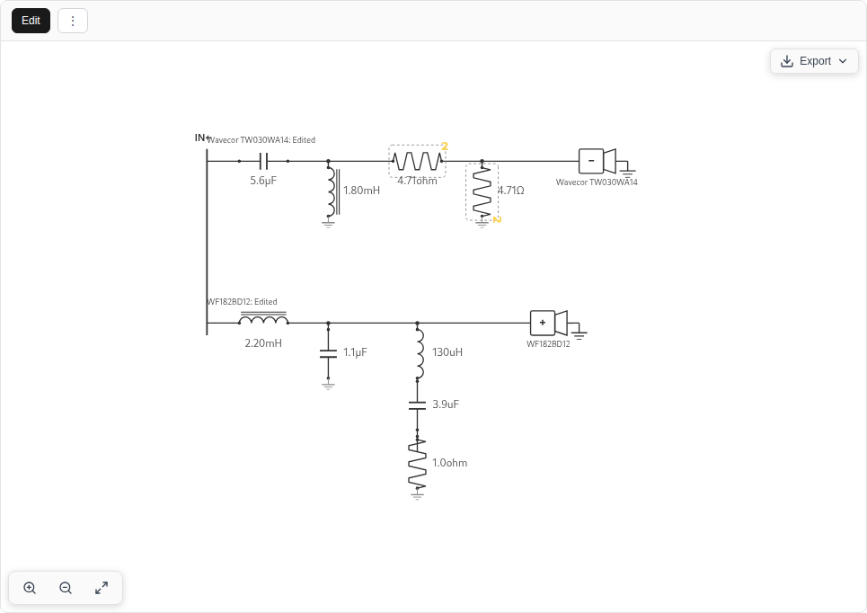
Click a passive component to change its value, test temporary open or short states, or adjust other supported properties, and select Split resistor when editing a resistor to distribute dissipation across multiple physical parts. Use the insertion controls to add a series or shunt element, and use the driver inspector to reverse polarity or combine same-model non-tweeter siblings into a shared branch wired in parallel or series (or split them back into separate branches). Where a design displays a shared filter bus feeding multiple drivers, you can edit its component values, parasitics, and bypass states directly or split the shared filter in the driver inspector when changing branch topology. Undo, Redo, and Undo All let you review edits, and saving keeps the settled draft.
You can manually design parallel passive crossovers with filter branches feeding the drivers. Within a branch, add series and shunt components, create parallel arms, and add multiple series components within an arm. These controls allow custom filters and correction networks without running Auto-Solve. The editor uses defined branch connections and wiring groups. It does not provide unrestricted wiring between arbitrary nodes or floating connections between driver branches.
Export options include PNG and SVG schematic images, passive SPICE text netlists (Show Netlist and Import Netlist for passive R, L, and C circuits matching the design's driver-branch count, omitting DSP stages), and portable complete netlist ZIP bundles. Export complete netlist packages the passive structure, DSP channel processing, and FIR assets together, and Import complete netlist lets you map each imported branch to the design's driver profiles.
6.1 Passive Components
The calculation uses the driver's complex impedance, including enclosure or coupled-chamber loading where applicable. Inductor winding resistance and capacitor series resistance affect the result. Estimated parasitics are useful starting points, but the parts you buy may have different values. The manual editor's component stock tables are separate from Auto-Solve's snapping stock series, so manual part entry is never forced into solver snap increments. Electrical filter order does not specify the final acoustic slope. The driver's own response, impedance, baffle, and phase all contribute. Review both the individual driver curves and their sum.
6.2 Network Calculation
Supported branches are evaluated as cascaded two-port networks using ABCD matrices. Each section describes how voltage and current pass through its components. Multiplying the matrices gives the complete branch at each frequency. The driver's complex impedance $Z_L$ terminates that chain in the transfer and input-impedance equations below.
Branches connected to a common amplifier are combined according to their wiring. Parallel or series multi-driver wiring groups and shared filter buses are solved with their actual electrical loading. The supported circuit model is not a general-purpose SPICE simulator for arbitrary active devices or floating connections between branches. Check the branch assignments as carefully as the component values when importing a netlist.
6.3 Correction Networks
Zobel networks reduce impedance variation over a useful band. Resistive pads reduce level, and resonant networks can reduce a peak or shape a crossover transition. A notch containing a resistor has finite impedance at resonance. Its depth depends on the surrounding circuit and load. A series element made from an inductor and resistor in parallel can provide baffle-step compensation. Choose its values against the modeled response rather than assuming every cabinet needs the same amount of attenuation.
6.4 DSP signal flow and amplifier channels
DSP applies mathematical filters to audio samples before amplification. Its gain, delay, and frequency shaping affect the voltage that reaches a passive network or a directly connected driver. A hybrid crossover keeps both digital processing and passive parts in the same design. Their order in the signal path is shown below.
Input → channel DSP → amplifier → passive branch → driver → acoustic field
                              └→ another passive branch on the same channel
The saved filter lane belongs to an amplifier channel. Branches sharing that channel receive the same DSP signal and present one combined load to that amplifier. Separate channels can have different gain, delay, and filters. An empty lane has transfer 1, preserving passive behavior unchanged. A bypassed stage preserves the blocks but applies no processing. When a saved design carries shared input-stage processing ahead of all channels, LoudspeakerLab evaluates it before channel lanes, checks it during device changes, and includes it in exports.
Select DSP / active stage to choose a device and assign its outputs. In the schematic, the purple plus controls insert DSP blocks before or after an existing block. Click a block to edit it. The inspector changes its frequency, gain, delay, shape, or other supported settings. Enabled bypasses one block without deleting it. Blocks run in their displayed order, which matters for the intermediate headroom check.
Parametric EQ changes a selected band, while low and high shelves adjust the balance toward either end of the spectrum. A notch reduces a narrow region, and an all-pass changes phase while preserving magnitude. High-pass and low-pass blocks divide the operating bands, with gain and delay setting relative level and arrival time. FIR blocks can use generated crossover filters, imported coefficients, or an editable group. The device profile determines which choices the hardware can reproduce.
To import a FIR, insert Imported FIR and choose its impulse file in the inspector. The supported files are WAV and text. Check the reported sample rate and tap count before using it. For a FIR group, add the member filters, choose Generated filter phase, and set Group taps. More taps use more device memory and can add delay. Section 6.6 explains the phase and delay calculations.
At frequency $f$, enabled blocks multiply:
$c(i)$ is driver $i$'s channel, $\sigma_i$ its wiring sign, $R_i$ its prepared acoustic response, and $G_i$ the propagation factor for position and listening distance. A rear-open cone's own front/rear sign is already inside $R_i$. It must not be added again as a second branch. Its electrical branch still needs its own measured impedance and channel assignment.
Gain $g$ dB gives $H_g=10^{g/20}$. Delay $\tau$ seconds gives $H_\tau=e^{-j2\pi f\tau}$: its magnitude is 1 but its phase changes with frequency. At 1 kHz, a 0.25 ms delay is −90°. Delay is not the same as reversing polarity, which multiplies pressure by −1 at every frequency.
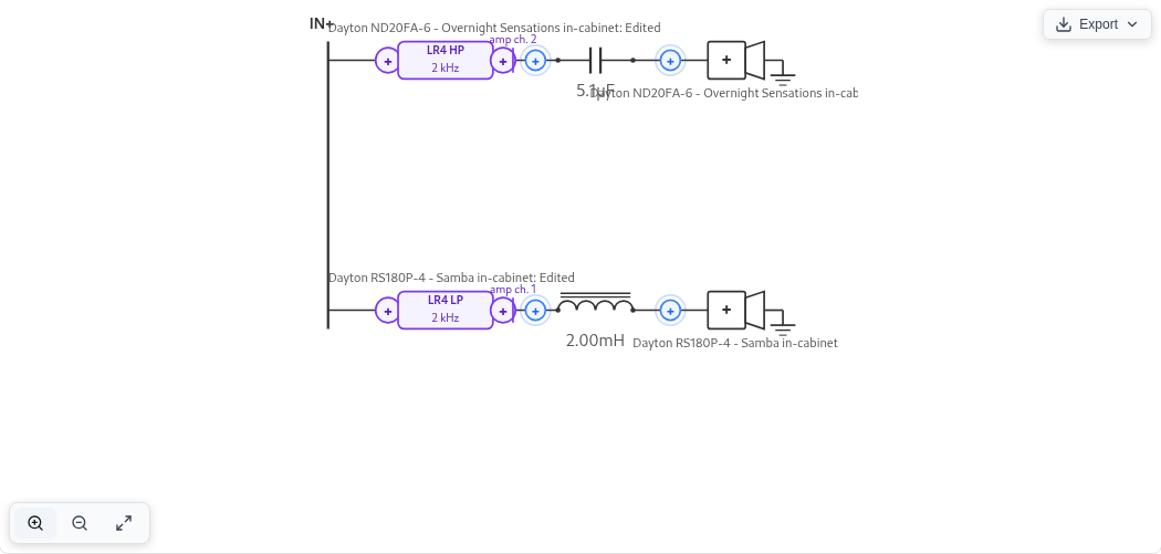
Read the digital IIR and FIR equations
6.5 Digital biquads and crossover shapes
A biquad uses the current sample, two previous input samples, and two previous output samples:
Its frequency response at sample rate $F_s$ is
These digital filters are evaluated at the device's sample rate. An analog filter with the same nominal cutoff does not give exactly the same curve, especially near Nyquist ($F_s/2$). For the RBJ coefficient formulas below, define $u=\cos(2\pi f_0/F_s)$, $v=\sin(2\pi f_0/F_s)$, and $\alpha=v/(2Q)$. Larger $Q$ makes a resonance or notch narrower. Divide all six raw coefficients by $a_0$ before evaluation.
| Filter | Raw $(b_0,b_1,b_2)$ | Raw $(a_0,a_1,a_2)$ |
|---|---|---|
| Second-order low-pass | $((1-u)/2,1-u,(1-u)/2)$ | $(1+\alpha,-2u,1-\alpha)$ |
| Second-order high-pass | $((1+u)/2,-(1+u),(1+u)/2)$ | $(1+\alpha,-2u,1-\alpha)$ |
| Notch | $(1,-2u,1)$ | $(1+\alpha,-2u,1-\alpha)$ |
| All-pass | $(1-\alpha,-2u,1+\alpha)$ | $(1+\alpha,-2u,1-\alpha)$ |
| Peaking EQ, $A=10^{g/40}$ | $(1+\alpha A,-2u,1-\alpha A)$ | $(1+\alpha/A,-2u,1-\alpha/A)$ |
An all-pass changes phase while keeping unit magnitude. Peaking EQ raises or lowers a band. A shelf changes the level toward one end of the spectrum. The shelf slope control governs how quickly that transition occurs. For a shelf, replace $\alpha$ with
where $S$ is the shelf slope parameter. The implemented raw low-shelf coefficients are
For the high shelf:
First-order sections use $K=\tan(\pi f_0/F_s)$ and $a_1=(K-1)/(K+1)$. Low-pass has $b_0=b_1=K/(K+1)$. High-pass has $b_0=1/(K+1)$ and $b_1=-b_0$. In both cases $a_2=b_2=0$. The Audio EQ Cookbook gives the underlying digital-filter formulas.
Higher-order crossover blocks cascade sections. The order is the requested slope divided by 6. 24 dB/octave means fourth order. This describes the filter's stopband trend, not the final acoustic slope after the driver is included.
- A Butterworth filter has a flat electrical passband. For order $N$, the following equation gives the quality factors of its second-order sections.
$$Q_m=\left[2\sin\!\left(\frac{\pi(2m+1)}{2N}\right)\right]^{-1},\qquad m=0,\ldots,\lfloor N/2\rfloor-1.$$Odd orders add a first-order section.
- A Linkwitz–Riley filter uses two identical Butterworth filters of order $N/2$ in series. Supported orders are 2, 4, 6, and 8. Each branch is −6 dB at crossover. A flat acoustic sum still requires appropriate polarity, timing, and driver responses. The electrical name does not guarantee it.
- A Bessel filter emphasizes a smooth group delay near the passband. Orders 1–8 use fixed section $Q$ values and frequency scales normalized to the −3 dB cutoff. High-pass sections use reciprocal frequency scales.
6.6 FIR filters: actual taps, phase, and latency
A finite impulse response (FIR) filter is a list of coefficients, or taps:
The plotted response uses the actual FIR coefficients, including the phase they produce. A symmetric nonzero core of $M$ taps has delay $(M-1)/(2F_s)$, apart from phase flips at zeros. Thus 1,025 symmetric taps at 48 kHz add about 10.67 ms. Group delay describes the delay of a narrow frequency band, with constant group delay indicating the same delay across frequencies. A long filter can describe a sharper low-frequency transition but consumes memory and adds latency. Linear-phase filtering can also place ringing before the main impulse peak.
A generated crossover FIR samples its target magnitude from zero frequency through Nyquist, then uses frequency-sampling synthesis and a Hann window. The window limits truncation ripple but changes the achieved curve. The core length is odd. An even requested allocation gets a trailing zero. That zero consumes storage but does not increase the core's group delay.
A FIR group combines editable filters into one allocation. Linear phase synthesizes the product magnitude. An all-pass cannot be included in this mode because its purpose is phase. Preserve filter phase filters a unit impulse through the requested IIR sections and retains the finite result, so truncation error depends on the allocated length. Gain and explicit delay are included. Diagnostics compare the resulting coefficients with the target.
Imported FIRs retain their level, timing, phase, and coefficient sequence. Import does not silently normalize, trim, center, resample, or make them symmetric. Resampling is an explicit operation, using polyphase resampling with amplitude adjustment for the changed sample density. An imported asymmetric impulse need not have constant group delay.
When imported and generated FIR filters share a group, their impulses are convolved:
The available tap count must hold the imported filters before adding a generated filter. An insufficient allocation is rejected. Any padding is placed at the end. Imported phase remains intact even if the generated part uses linear phase. If the device rounds its coefficients, the displayed result uses those rounded values.
Older saved FIR designs keep their original filter interpretation unless the owner explicitly upgrades them. Check the settled result and the exported setup after an upgrade. The saved coefficients provide a reference for a device already running the old settings. Compare the old and updated responses before replacing them on the hardware.
6.7 Matching filters to a DSP device
A DSP device may limit its filter types, channel routing, delay steps, and FIR length. LoudspeakerLab tracks 14 device profiles and distinguishes four capability states for each processing block: a known hardware limit, an unknown limit, an unsupported block, or an unbounded software limit. Digital biquad filters are evaluated at the selected device sample rate with exact mathematical parity between instant previews, settled calculations, and exported device coefficients. Select the device and sample rate before judging the final response, because if a crossover exceeds a channel's available filter slots, saves are blocked rather than silently dropping filters on hardware export.
Gain and delay are rounded to the device's available steps. For a step size $\Delta$, a setting $x$ becomes $x_{\rm set}=\Delta\,\operatorname{round}(x/\Delta)$. At an exact half-step, the value rounds away from zero. A delay measured in whole samples follows $\tau=N/F_s$. Check the selected device's specifications for other step sizes. Unknown hardware precision or interpolation remains an estimate.
For each channel, the headroom check examines the gain after every stage:
A positive peak means some intermediate signal can exceed input full scale even if a later cut reduces the final output. This frequency-domain headroom check does not simulate clipping, limiters, arbitrary waveform peaks, or compression.
Open the schematic’s Export menu and choose DSP config to review or download the device setup ZIP package. Native configuration exports generate device-ready files for miniDSP devices (2x4 HD, Flex, Flex Eight, Flex HT, and SHD series with miniDSP biquad sign conversion and FIR files), CamillaDSP (YAML fragments and FIR files), and Equalizer APO with Peace (configuration text and WAV FIR files). Other supported profiles (Behringer DCX2496, dbx DriveRack PA2, the t.racks DSP 204 and 408, Dayton Audio DSP-408, Hypex FusionAmp FA series, and Generic) emit a reference setup sheet listing exact manual gain, delay, polarity, routing, and filter parameters alongside reference FIR files where applicable. Every package flags any manual steps or omitted processing, so check the setup sheet and keep it with the saved revision.
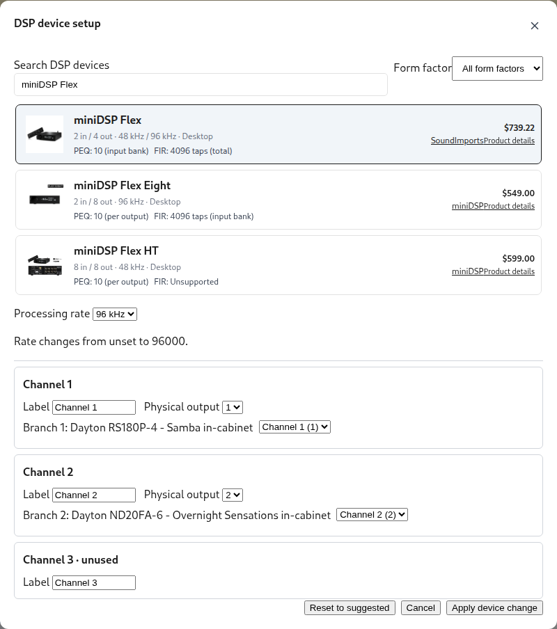
6.8 Channel impedance, output limits, and sensitivity
Separate amplifier channels do not share one parallel input load. Each sees the branches connected to its own output. Independent parallel branches combine as complex admittances, as shown below. A shared passive network must instead be counted according to its actual electrical connection.
The impedance chart shows the load for each amplifier channel. The active-design headline reports the lowest load on any channel. Two independent 8 Ω channels each see 8 Ω. Two 8 Ω branches in parallel on one channel present 4 Ω.
For RMS channel voltage, $I_c=V_c/Z_c$ and real input power is $P_c=|V_c|^2\operatorname{Re}(1/Z_c)$. Resistor heating uses $|I_R|^2R$. The output estimate compares predicted cone motion, component heating, driver ratings, and amplifier limits for each channel. Two branches wired to one channel are one amplifier load.
DSP gain changes the meaning of sensitivity because the response at 2.83 V at its input includes the chosen gain setting. That number is not the raw driver's efficiency. Maximum SPL is more useful for comparing active designs when their amplifier, excursion, and thermal assumptions match. Boost still consumes cone travel and amplifier voltage. You can edit the filters manually or use Auto-Solve for a supported active or hybrid layout, then check the completed curves and loads.
6.9 Preview and completed results
While you adjust passive networks, shared electrical graphs, coupled cabinet fields, digital biquads, or parametric FIR groups (without all-pass filters in linear-phase mode), the editor computes an immediate preview directly in your browser. Imported custom FIR impulses wait for the full server calculation rather than using a local estimate. Roughly 0.8 seconds after you pause editing, LoudspeakerLab updates the plots with the authoritative settled calculation, which is especially important for close listening distances, off-axis contours, and complex coupled enclosures. Saves and hardware DSP exports always compile the full authoritative design and never export from the fast browser estimate.
For a practical design, first choose the physical sources and their measured or modeled radiation. Then assign amplifier channels, choose the DSP profile and rate, and add filters. Check summed level, phase, full front/rear patterns, each amplifier load, excursion, and headroom. Wait for the settled result before judging a change. Export the setup, apply any listed manual settings, and measure the assembled speaker to verify the prediction.
6.10 Complete an active or hybrid design
- Select the physical sources, cabinet, measurement profiles, and listening position.
- Enable DSP, choose a device and sample rate, and map its outputs to the driver branches.
- Add channel filters yourself, or save the channel layout and use Auto-Solve. Inspect the individual driver curves, their sum, gain, delay, and polarity.
- Wait for the completed calculation, then inspect directivity, each amplifier load, excursion, maximum SPL, and headroom.
- Export DSP config, apply the listed manual settings, and measure the assembled speaker with that configuration.
Changing the device preserves the editable filter design. The preview identifies processing that the new profile cannot reproduce or that needs manual setup. An incomplete export package lists omitted processing. Check its setup sheet before assuming the hardware matches the plot.
7. Response, Directivity, and Listening Position
The system response combines the drivers as complex pressures. That retains both their magnitude and phase before the sum is taken. Equal levels can reinforce one another or nearly cancel, depending on their relative phase. Driver position, cabinet radiation, polarity, and filtering all contribute to that relationship.
7.1 Summing the Drivers
Drivers can reinforce or cancel one another where their operating bands overlap. A smooth sum on the reference axis can still produce a narrow or tilted vertical lobe. Check the horizontal and vertical plots as well as the main response. A polarity change can improve one handoff while altering the lobe on the other side of the axis.
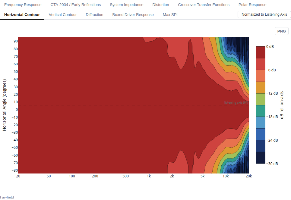
7.2 Listening Distance and Angle
Listening-position controls separate the standardized far-field speaker reference from your specific listening seat. System response, CTA-2034 curves, contours, Directivity Index, Sound Power, and Preference Rating all share one exact asymptotic far-field reference, whereas choosing a finite listening distance (from 0.5 to 10 metres, or farfield) adds an explicit Listener point response reflecting each driver's actual path length and off-axis angle at your seat without folding $1/d$ distance loss into far-field sensitivity or Preference Rating. In Show environment, the acoustic scene shows the cabinet, driver arrival paths, and an expanding 3D radiation balloon whose radius scales with listening distance while normalizing the radiation pattern at each distance, along with mobile WebXR and iOS gyroscope AR directivity viewing. Symmetric layouts preserve bilateral horizontal symmetry, continuous vertical unfolding prevents rear-hemisphere contour jumps, and preview curves fade to half opacity beyond a driver's measured coverage.
The immediate crossover preview uses a far-field approximation. A finite-distance result can change when the completed calculation arrives. Inspect the settled result before saving conclusions about a close listening position. This matters most when driver spacing is large relative to the listening distance.
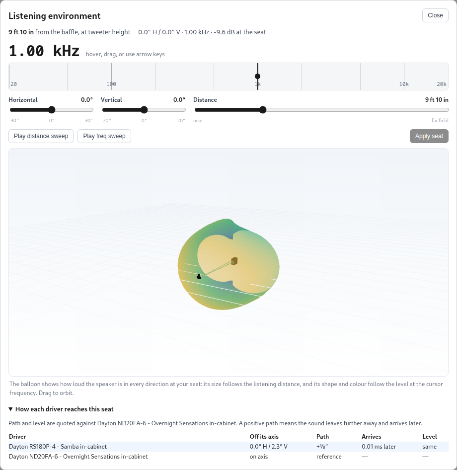
Show environment has a frequency control for the balloon and a distance control for the listener. A prepared complex field combines each driver with its settled crossover transfer, adds propagation once, and sums pressure before taking its magnitude. A legacy design uses a labeled magnitude-only approximation. Its appearance cannot establish front-to-rear phase or a measured full sphere.
7.3 CTA-2034 Curves
The CTA-2034 view summarizes modeled radiation using curves defined by the CTA-2034 measurement standard. These are predictions based on the driver data and model assumptions. They are not a physical compliance measurement. The angular coverage and measurement basis are recorded with the design rather than inferred from the smoothness of the plot.
- On-axis response describes the reference direction.
- Listening Window averages nine directions near the reference axis.
- Early Reflections combines angular groups associated with typical floor, ceiling, front, side, and rear reflections.
- Sound Power estimates radiation into full space from weighted angular responses. The completed calculation uses ring weights rather than a dense measured spherical scan.
- ERDI and SPDI subtract Early Reflections and Sound Power from the Listening Window. They show how radiation away from the listening window changes with frequency.
- Predicted In-Room response combines Listening Window, Early Reflections, and Sound Power in linear power with weights of 0.12, 0.44, and 0.44.
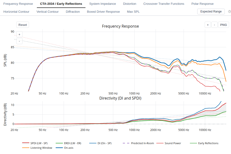
Read the curves together. A sharp directivity change near a crossover can remain visible in the reflected sound even when the on-axis response is smooth. The quality of the prediction depends particularly on the available off-axis measurements. A contour can reveal a narrow null that is less obvious in an averaged curve.
7.4 Preference Rating
The Preference Rating adapts Olive's regression model. It combines response smoothness, narrow-band deviations, and low-frequency extension. LoudspeakerLab changes the intercept and also shows a subwoofer-assisted variant. Its purpose is to summarize particular response features, not to replace the response and load plots.
The score is useful for comparing revisions under consistent assumptions. It is not a listening-test result, and values from another program may use different equations or conventions. “PR with Sub” represents the scoring assumption for bass support. It does not simulate a particular subwoofer and crossover.
7.5 How the summary curves are formed
At each frequency and direction, the individual driver pressures add as complex numbers: $p_{\rm total}=\sum_i p_i$. A +3 dB rise from two sources is not automatic. Their relative phase determines whether they reinforce or cancel. At a finite listening distance, each source has a slightly different path length and viewing angle. A path difference $\Delta r$ adds phase $-2\pi f\Delta r/c$ and changes the relative distance level. This is why listening height can change crossover lobing.
First add the driver pressures within each direction. The angular summaries then average the resulting sound energy across their selected directions. This is different from averaging decibel values or adding the drivers after their angular curves have been averaged. The equation below gives that energy average for levels $L_a$ and normalized weights $w_a$.
Listening Window uses nine directions around the reference axis. Early Reflections groups directions that commonly feed the floor, ceiling, and front, side, and rear walls. Sound Power estimates the total radiated energy by weighting directions for the area of sphere each represents. For an open-baffle design, its rear-angle measurements or predictions must be included. ERDI = Listening Window − Early Reflections and SPDI = Listening Window − Sound Power. A rising directivity index means less energy is sent away from the listening region at that frequency.
Predicted In-Room response uses 12% Listening Window, 44% Early Reflections, and 44% Sound Power in linear energy, followed by conversion back to dB. It is a useful spectral trend across typical directions. It has no room dimensions, speaker placement, or wall materials, so it cannot predict room modes or the response at your seat. The Preference Rating (PR) is an adapted statistical summary of response smoothness, narrow peaks and dips, and bass extension. The following equation gives its terms.
$SM$ describes how smoothly a response follows a broad frequency trend. $NBD$ measures smaller bumps and dips after half-octave smoothing. $F_{-6\rm dB}$ estimates low-frequency extension against a reference level. PR with Sub substitutes ideal extension to 14.5 Hz for this one bass term. It does not add a particular subwoofer to the design. The score is a comparison aid under common assumptions, not a listening test or a guarantee of preference.
8. Impedance and Output Limits
A small-signal response is only part of deciding how loudly a speaker can play. Driver ratings and cone travel can limit the useful output before the response shape becomes a problem. Passive components and amplifier channels add their own limits. Inspect those curves together before choosing the amplifier and physical parts.
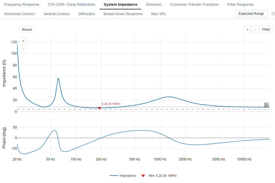
8.1 Power Handling
Thermal estimates use driver ratings, electrical transfer functions, and defined signal spectra. The component analysis estimates dissipation in the crossover. Its IEC-style and AES75-style profiles describe calculation assumptions, not completed standard measurement procedures. The model does not solve the changing voice-coil temperature and feed its resistance rise back into the complete response. It therefore does not predict thermal compression as a time-dependent process.
8.2 Excursion and Maximum SPL
Excursion estimates use the driver data and enclosure behavior to identify where the cone reaches its specified linear travel. In vented systems, below-tuning excursion is especially important. Missing or uncertain $X_{\max}$ and power ratings limit what the maximum-SPL result can establish. Check the supplier’s stated excursion convention before comparing limits from different driver profiles.
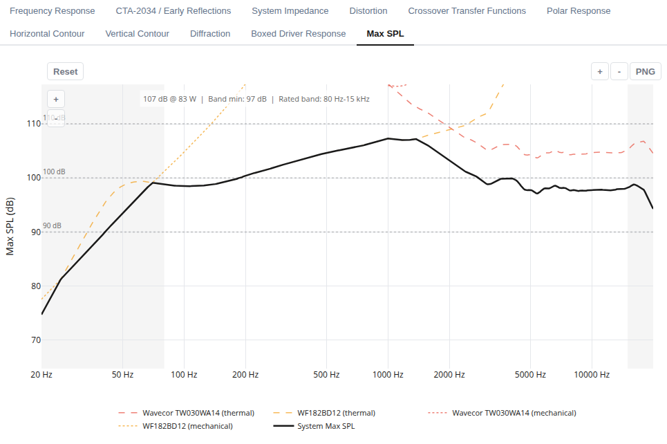
The maximum-SPL chart evaluates passive enclosures, coupled multi-aperture chambers (vented, passive-radiator, and shared-chamber builds), shared-filter circuits, independent-source directional pairs (dipole, bipole, and cardioid), and multi-channel active or hybrid DSP layouts consistently by combining driver thermal ratings, cone excursion, passive component heating, and per-channel amplifier limits. Treat it as a design estimate. It does not certify distortion-free playback, reproduce the full AES75 test, or account for every high-level effect such as port compression, magnetic saturation, or suspension nonlinearity. When an amplifier or driver rating is unknown, LoudspeakerLab explicitly reports that limit as unestablished rather than inventing a ceiling.
8.3 Amplifier Load and EPDR
Inspect impedance magnitude and phase together. Low impedance increases current demand, and a reactive phase angle can increase output-device dissipation in a class-AB amplifier. Equivalent Peak Dissipation Resistance, or EPDR, expresses that modeled peak dissipation as an equivalent resistive load. It is not the speaker's DC resistance or a universal amplifier-compatibility rating. Amplifier topology, protection, supply limits, and the signal all affect actual operation.
8.4 Resistor Networks
A crossover resistance can be realized with several physical resistors to share dissipation. LoudspeakerLab lets you use the Split resistor action in the component inspector alongside automatic physical resistor network tracking in thermal estimates, carrying those physical combinations directly into the schematic and parts list. Inspect the physical parts and power estimates, not just the aggregate resistance. Installation, spacing, and ventilation affect real resistor temperatures.
8.5 Interpret the available headroom
If the predicted peak cone travel at a reference drive is $x_{\rm ref}$, the linear excursion headroom before reaching $X_{\max}$ is
This relationship assumes that cone travel scales with voltage. A 6 dB bass boost uses about twice the voltage and cone travel. Read the entire Maximum SPL curve because a high headline value can coexist with a much lower bass limit. With multiple amplifier channels, check which driver or channel reaches its limit first.
9. Auto-Solve
Auto-Solve develops a crossover for the drivers, cabinet, and listening settings in your draft. For a passive design, it searches supported circuit arrangements and their component values. For an active or hybrid design, it uses the saved amplifier channels and DSP device to divide the filtering between channel processing and supported passive handoffs. You choose the goals and constraints, then receive an editable result with the final parts or filter coefficients used in its plots.
Use it when the drivers and cabinet are chosen but the filtering is still undecided. A run can explore a different balance of response, dispersion, amplifier load, and complexity. The result remains a candidate to inspect against your own requirements. Comparing it with another run or a manually edited revision often makes the tradeoffs clearer.
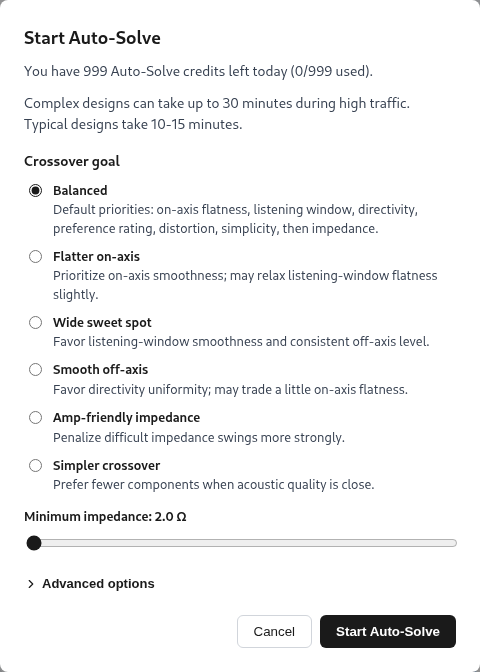
Save the draft before opening Auto-Solve, including channel assignments and FIR groups if the design is active. Choose a goal and minimum impedance, then open Advanced options if you need different priorities, crossover targets, or allowed passive networks. Start the search once those settings describe what you intend to build. The status page reports progress, and the completed candidate opens with its schematic and calculated results. Review that candidate before saving or publishing it.
9.1 What the search designs
The crossover must work with each driver's measured response and changing impedance. Its electrical filter combines with the driver's existing acoustic rolloff, cabinet effects, placement, and phase. Auto-Solve evaluates those relationships together, including how the driver outputs add around each crossover region, and supports prepared coupled-chamber and open-panel constructions as well as conventional boxes. Coupled topology discovery supports up to two coupled sources per shared chamber, while shared chambers with three or more sources remain supported for manual editing and fixed-circuit evaluation. Every candidate undergoes an authoritative acoustic review before finalization, and the finished schematic and plots preserve your authored driver order and branch identities.
Auto-Solve keeps the selected drivers and cabinet as its design context. In an active design, it also keeps the saved channel assignments, device, sample rate, and physical outputs. It can replace passive parts for supported internal handoffs and add its own output processing while retaining other authored processing. Subwoofer-only systems and imported fixed netlists evaluate directly without running a full topology search, and failed or interrupted solver runs do not consume a daily Auto-Solve allowance. Driver selection, cabinet resizing, and channel reassignment remain decisions you make through their own controls.
The completed plots describe the final available component values. This matters because a smooth result with an ideal value is useful only if the circuit still performs well with the parts you can use. You receive the selected schematic and its calculated behavior together. Supplier tolerances and losses still need to match the assumptions closely enough for the intended build.
9.2 Priorities and Constraints
Start with a named goal that is close to what you want from the speaker. Advanced options lets you change the priority order when a preset does not suit the project. The same goal can lead to different choices with a different driver set, cabinet, or amplifier layout. Read the preset as a preference for the search, then judge its effect in the completed curves.
- Balanced gives you a starting compromise among the available acoustic and electrical goals.
- Flatter on-axis emphasizes the response straight ahead.
- Wide sweet spot favors a smooth response across the listening window.
- Smooth off-axis emphasizes consistent dispersion through the crossover regions.
- Amp-friendly impedance gives more attention to the electrical load.
- Simpler crossover favors fewer components when the acoustic results are close.
Minimum impedance is a separate constraint, so set it for the amplifier you intend to use. A passive design presents one combined load, while an active design has a load for each amplifier channel. The hybrid solve checks each channel over the complete analysis grid, including a channel driving a single driver directly. Inspect magnitude and phase in the result, since a minimum magnitude alone cannot establish that every amplifier will be comfortable with the load.
These goals can conflict. Extra attenuation may smooth the response while reducing sensitivity. A correction network may suppress a peak while adding cost and dissipation. An impedance constraint can rule out an otherwise attractive acoustic result. Distortion measurements can inform the design where suitable data are available, but a missing distortion measurement cannot become a verified low-distortion result.
A preset expresses which tradeoffs you would like the search to favor. It cannot make incompatible drivers meet every goal at once. If two priorities compete, compare the completed curves, loads, output limits, and actual parts. Keep the candidate that suits the project rather than assuming the highest single metric makes the best speaker.
9.3 Targets and Manual Networks
Advanced options let you guide the handoff between adjacent drivers with available crossover-frequency and slope targets. The target controls show the usable ranges derived for the selected drivers. Choose a handoff where both drivers have suitable response, dispersion, and output capacity. A target cannot make a driver behave well outside its usable band.
You can also restrict the available correction networks. This is useful when you want a simpler construction or wish to avoid a particular type of network. Restrictions reduce the alternatives the search can use, so review their effect on the response and load. A requested electrical order does not guarantee the same acoustic slope after the driver and cabinet are included.
You can also enter a supported passive network and evaluate it without running Auto-Solve. SPICE-style passive text netlists and portable complete netlist bundles represent the supported circuit structures and DSP configurations. They do not provide compatibility with arbitrary SPICE active devices, commands, or floating cross-branch topologies. Importing asks you to map driver branches, so review those bindings before comparing its response with another tool.
9.4 Review the selected circuit
- Check the inputs. Confirm the measurement profiles, enclosure, driver positions, listening axis, and data assumptions. Those inputs determine which physical system was searched.
- Read the acoustic result. Compare the individual driver curves, their sum, listening window, and contours. Look for a sensible handoff and acceptable behavior away from the axis.
- Read the electrical and output limits. Inspect impedance, component dissipation, and Maximum SPL across frequency. Check the actual polarity, component values, and ratings.
- Review the build. Check part availability, missing prices, and physical requirements. Save an editable draft and use the editor to investigate specific changes.
- Validate a prototype. Measure the assembled speaker and refine the design against those measurements. Publish the version you intend others to inspect.
For a useful comparison, keep the drivers, cabinet, and listening settings fixed while changing one search preference. Compare the resulting circuits and curves together. A higher preference estimate or a flatter axis curve can coexist with a less suitable impedance, lower sensitivity, or a more complicated build. Save the relevant candidate rather than relying on a metric copied from a previous run.
Auto-Solve uses a stochastic numerical search, so another run can find a different candidate. It does not prove that its circuit is the global optimum, and it cannot fix inaccurate measurements or missing physics. Its value is finding and evaluating plausible alternatives within the supported design space. The completed model and a measured prototype remain the evidence for the result.
9.5 Active and hybrid Auto-Solve
Set the amplifier channels and device before starting an active solve. Each channel needs a contiguous run of frequency bands, such as a woofer on one channel and a midrange plus tweeter on another. A channel with one driver uses active filtering without a passive crossover. Supported independent drivers on the same channel need passive handoffs between their bands. The channel processing handles the handoff to drivers on other amplifiers, and every load is checked against the impedance constraint.
For that three-way example, the woofer channel receives a low-pass, while the midrange and tweeter channel receives the matching high-pass. The midrange-to-tweeter handoff is made with passive parts after their shared amplifier. Auto-Solve also adjusts channel gain, delay, polarity, and a limited set of EQ filters against the calculated response. Existing input processing, other authored output blocks, and shared passive circuits keep their intended structure. A shared or dependent passive network is evaluated as authored rather than redesigned as separate independent branches.
To use FIR for a channel, add a FIR group and choose its tap allocation and phase mode before saving the draft. Auto-Solve places its crossover and EQ members inside that group without discarding your authored members. The group produces one finite impulse using the selected device's coefficient format, and those coefficients drive both the plotted response and export. Low-frequency transitions need enough taps, and an inaccurate realization can require a larger allocation or a higher crossover frequency. Linear-phase FIR adds latency, so the solve checks the attainable delay and actual complex sum when aligning it with IIR channels.
The automatic EQ uses a bounded set of editable filters rather than trying to invert every feature of the acoustic response. It does not boost a deep cancellation into a useful source or promise zero acoustic phase for the complete speaker. Interleaved channel bands, missing assignments, unsupported devices, or more than one enabled FIR group on a channel can prevent a solve from starting. Read the error or warning, correct the layout, and save it before trying again. After a successful run, inspect each channel's load, headroom, full response, and export instructions before applying the settings to hardware.
10. From a Design to a Prototype
10.1 Recommended Workflow
For open panels and constructions, first choose modeled driver input or complex measurements of the target assembly (Section 5.14). Review rear radiation and declared limits. For active designs, choose channel routing and the DSP device, then follow Section 6.10. The same checks apply to conventional passive designs.
- Select drivers and inspect their measurement sources, usable bands, and missing data.
- Choose an enclosure alignment. Check volume, tuning, excursion, and physical clearances.
- Set the driver positions and baffle geometry. Review diffraction and the intended listening axis.
- Enter a crossover or run Auto-Solve with the saved channel layout. Compare the individual responses, their sum, directivity, and amplifier loads.
- Review output limits, evidence, assumptions, and parts. Build a prototype, measure it, and use the results to refine the design.
Published designs have public pages where other users can inspect the results and create their own remixes. A remix creates an editable copy. Publication does not establish that the speaker has been built or measured. Build notes and measured results can provide that additional evidence when the author shares them.
10.2 Read Expected Range
Select Expected Range on the Frequency Response, CTA-2034 / Early Reflections, or System Impedance tab to generate and overlay the sensitivity band on demand for a saved, completed design. Its samples vary driver response, bass assumptions, directivity, impedance, acoustic-center depth, and component values, while a residual floor captures remaining uncertainty. Because Expected Range belongs to the saved circuit and listening axis, the toggle disables itself while unsaved crossover edits or modified listening settings are active until you save.
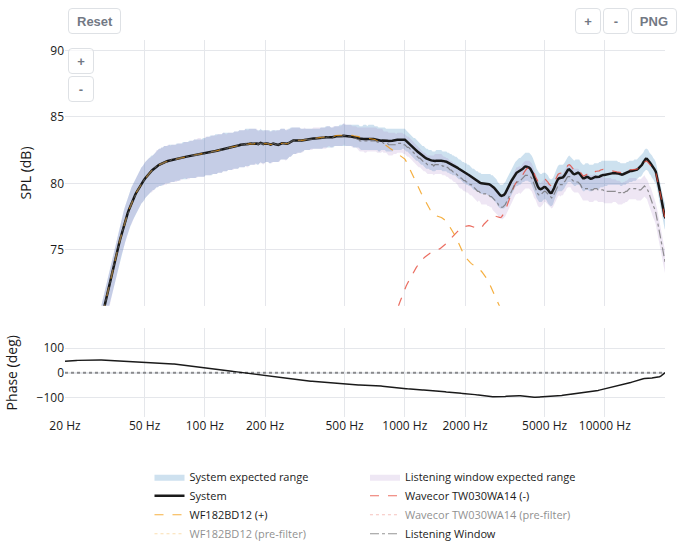
The central band runs from the 10th to the 90th percentile of these modeled outcomes. These percentiles describe the chosen assumptions. They do not give a calibrated probability that a finished speaker will fall inside the band. Use wide regions to decide where better measurements or a prototype check would be most useful.
10.3 Design Evidence
The design evidence score summarizes data provenance, directivity coverage, low-frequency modeling, and data integrity. Their current weights are 55%, 25%, 15%, and 5%. The overall score is capped at eight points above the lowest individual driver provenance score. This score describes the basis for the prediction. It does not rate workmanship, sound quality, or the success of a physical build.
10.4 Review assumptions, parts, and build documents
Select View assumptions detail to inspect the calculation basis stored with the result. It includes measurement sources, phase treatment, acoustic-center choices, directivity estimates, enclosure losses, and power assumptions. A strong evidence score does not turn an estimated center depth or missing rear curve into a measurement. Check the entries most relevant to the change you are comparing.
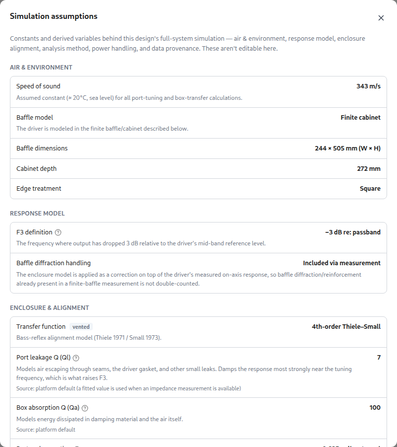
Open Parts List to inspect drivers, passive parts, and any selected passive radiator, pre-built cabinet, or DSP device. LoudspeakerLab matches passive components across 12 component vendor catalogs and drivers across 11 driver vendor catalogs, estimates regional costs across five regions (US, EU, UK, CA, and AU) with currency conversion, and provides bulk retailer cart links where supported. Design browsing also supports cost-per-Preference-Rating comparisons alongside total cost estimates. Resistor arrays list the physical parts as well as the equivalent resistance, and missing prices remain visible so a total with a plus sign indicates an incomplete estimate.
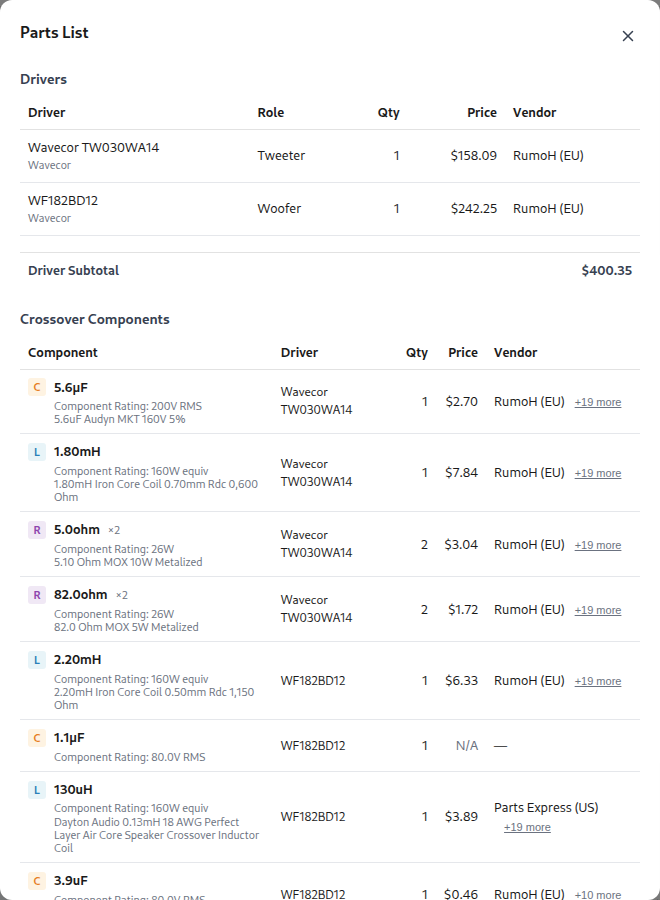
Check resistance, capacitance, inductance, winding resistance, capacitor losses, power rating, and mechanical fit against the supplier’s data. Browse Accessories for available passive radiators, pre-built cabinets, and DSP products. The region control changes shopping links and currency, but it does not establish live warehouse stock. A part that matches the nominal value can still have a different loss or rating from the one used in the calculation.
The Build Sheet and Cut sheet provide the available cabinet views, panel sizes, cutout locations, and material layout. Plot PNG and schematic PNG or SVG Export provide images for notes or sharing. The passive SPICE netlist, portable complete netlist ZIP, and DSP config provide the supported electrical and processing setup. Keep these files with the driver-profile identities and saved design settings.
10.5 Compare designs and listen to their tonal balance
Select Compare on a completed design and choose another draft you own or a public design. The comparison view overlays compatible curves, shows other views side by side, and pairs them with a table of response, bass, load, output, and cost metrics where available. The selected view stays in the URL so a comparison of public designs can be shared. Use the same listening settings and compatible input data when judging the difference. A curve based on in-cabinet measurements and one based on a specification sheet do not isolate the effect of the crossover.
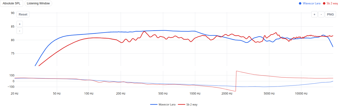
Select Listen to open the listening panel. It filters pink noise with the design’s listening-window frequency balance. Switch between Reference (flat) and Speaker to hear the tonal change. Headphones can make this difference easier to hear.
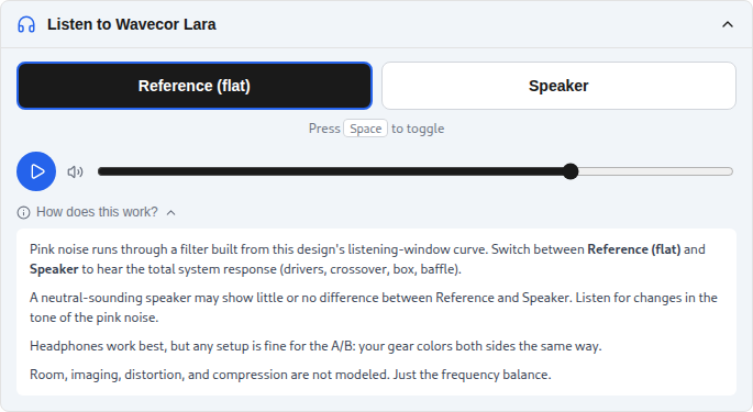
The listening demonstration represents the modeled frequency balance. It does not reproduce stereo imaging, room reflections, distortion, or high-level compression. It also cannot reproduce the physical speaker’s radiation pattern through headphones. Use it to hear broad tonal changes, then judge spatial and high-level behavior with the actual speaker.
10.6 Save, publish, remix, and verify
Save keeps the editable draft and its settings. Publishing creates a fixed public version. Share supplies the public link, and a project website link can point to your build notes. Other signed-in users can star or comment on the published design. Remix creates a new editable copy of a published version, crossover forking lets you branch a published crossover for alternative filtering, and published-design driver migration creates an editable migrated copy when swapping in a replacement driver. Staleness notices alert you when driver profiles or design inputs have changed relative to a saved curve.
Use Edit to change a design’s driver and cabinet inputs. Review the recalculated result before saving it. Delete removes a design you own after confirmation, so export any information you need to retain first. A published version remains fixed, so make a remix when you want to retain changes to it.
A draft’s cabinet finish can be saved with the design and rendered in 3D with baked ambient occlusion. Publication preserves and freezes the chosen finish. Changing the appearance while viewing a published design previews the look without saving a new cabinet specification. Remix the design when you want to keep a finish change.
Build a prototype and measure its response, impedance, and directivity. Compare those measurements with the prediction at the same drive level and listening reference. Use the differences to check driver samples, cabinet losses, port tuning, component values, and timing. Publication alone does not establish that a design has been built or measured.
Use the measurement instructions when preparing files and acquisition notes. The FAQ section covers individual questions about uploads, settings, accounts, and saved designs. If those pages do not answer your question, the Support page gives the available contact options. The accuracy studies compare particular predictions with measured speakers. Read their input data and test conditions before applying a result to a different design.
11. Compare LoudspeakerLab with other design tools
LoudspeakerLab keeps driver selection, cabinet sizing, crossover design, result review, and build documents in one browser project. That suits work where the cabinet, passive network, and DSP need to be considered together. Other programs provide more control over particular measurements, circuits, acoustic structures, or high-level studies. The comparisons below describe those documented differences without turning a feature list into an accuracy ranking.
11.1 What supports the comparison
LoudspeakerLab's documented capabilities and the BEM and cabinet-modeling comparison criteria were updated on November 19, 2026, while the competitor comparisons below use the developers’ manuals and feature lists checked on September 29 and 30, 2026 (listed in Section 11.11). They distinguish products and editions. A feature documented in LspCAD Pro is not attributed to its Standard edition. FINE X-over, FINE DSP, and FINEBox PRO are separate products. EASE SpeakerLab authors loudspeaker models, while other EASE applications perform room and coverage studies.
The statements about which program is a better fit are judgments based on the named task and documented controls. They are not rankings of sound quality or proof of greater acoustic accuracy. Missing documentation is not treated as proof that a feature is absent. No total score is assigned because the programs serve different purposes.
11.2 Feature comparison matrix
Read across a row using the criterion beneath its feature name. Equivalent documented functions use the same wording. Additional sentences identify verified differences or specific gaps in the evidence. Shared wording establishes comparable coverage, rather than identical formulas or numerical results. The source documents and product discussions explain the evidence.
- Leading means the tool supports the feature and has a clear documented advantage for that row’s criterion over the other verified workflows. Select the label to read the reason. It does not rank acoustic accuracy or rule out equivalent unverified support.
- Supported means the reviewed implementation or product documentation establishes the feature.
- Limited means the program covers part of the feature or provides a related workflow. The cell explains the difference.
- Not offered means the reviewed implementation or documentation excludes that function.
- Not verified means the reviewed sources do not establish support. It does not mean the feature is absent.
- Separate product means another license or application supplies the function.
Product and edition labels identify Pro restrictions and the specific FINE license, whose separate products share a column only for comparison. Angular import and interpolation have separate rows so one does not imply the other. AKABAK’s introduction establishes its broad solver scope but leaves several design-workflow features unverified. XSim entries distinguish classic XSim from the analog additions in XSim4 and use primary developer posts. Functions not established by those posts remain unverified. The labels describe coverage, not relative accuracy.
| Feature and comparison criterion | LoudspeakerLab | VituixCAD 3 | SoundEasy V31 | LspCAD 6 | FINE products | AKABAK | EASE SpeakerLab | XSim / XSim4 |
|---|---|---|---|---|---|---|---|---|
| Measurements and directivity | ||||||||
| Response and impedance importBoth acoustic response and electrical impedance must be importable. | SupportedIt imports frequency-response and impedance text files. | SupportedIt imports frequency-response and impedance text files. | SupportedIt imports frequency-response and impedance text files. | SupportedIt imports frequency-response and impedance text files. | SupportedFINE X-overIt imports frequency-response and impedance text files. | Not verifiedImport of measured frequency-response and impedance text files was not verified. | SupportedIt imports frequency-response and impedance text files. It also accepts measured impulse responses for source models. | SupportedIt imports frequency-response and impedance text files. |
| Built-in acoustic measurement captureThe software must acquire measurements, rather than only import them. | Not offeredIt uses measurements captured by other software. | Not offeredIt uses measurements captured by other software. Its FFT tool processes existing recordings. | LeadingIt captures acoustic response and impedance. It also controls a compatible turntable for automated 360° angular measurements. | SupportedStandard and ProIt captures measurements through bundled justMLS. Automated angular acquisition was not verified. | Separate productMeasurement capture requires the separate FINE R+D product. | Not verifiedBuilt-in measurement capture was not verified. | Not offeredIt uses measurements captured by other software. | Not verifiedBuilt-in acquisition was not verified. The documented workflow imports external measurements. |
| Thiele-Small parameter extractionThe comparison includes which driver parameters can be derived from measurements. | LimitedIt estimates resonance, resistance, damping, inductance, and regression compliance non-destructively from free-air impedance, and fits vented in-box impedance when box data are supplied. | SupportedIt derives resonance, resistance, damping, moving mass, and compliance volume using added-mass or sealed-box measurements. | SupportedIt derives resonance, resistance, damping, moving mass, and compliance volume using added-mass or sealed-box measurements. | Not verifiedParameter extraction from measurements was not verified. | Not verifiedParameter extraction from measurements was not verified. | Not verifiedParameter extraction from measurements was not verified. | Not offeredIt does not extract driver parameters from measurements. | Not verifiedThiele-Small parameter extraction was not verified. |
| Near-field and far-field response mergeThe comparison covers the splice and the available matching controls. | SupportedIt merges low-frequency and high-frequency responses. Cone and port data are combined and blended automatically with the gated response. | SupportedIt merges low-frequency and high-frequency responses. It exposes multi-source scaling and delay adjustment. It also matches delay automatically and adjusts blend width. | SupportedIt merges low-frequency and high-frequency responses. It exposes multi-source scaling and delay adjustment. Curves are merged at a selected frequency. Variable blend-width control was not verified. | SupportedIt merges low-frequency and high-frequency responses. It exposes level and delay matching for two curves. | Not verifiedNear-field and far-field response merging was not verified. | Not verifiedNear-field and far-field response merging was not verified. | Not verifiedNear-field and far-field response merging was not verified. | Not verifiedNear-field and far-field merging was not verified. |
| Phase and timing treatmentThe comparison covers measured phase, relative timing, and reconstructed phase. | SupportedIt preserves measured phase, matches shared timing references automatically from compatible measurements, models relative delay, and reconstructs minimum phase. | SupportedIt preserves measured phase and models relative delay. It can also reconstruct minimum phase. | SupportedIt preserves measured phase and models relative delay. It can also reconstruct minimum phase. | SupportedIt preserves measured phase and models relative delay. Built-in minimum-phase reconstruction was not verified. | SupportedIt preserves measured phase and models relative delay. Built-in minimum-phase reconstruction was not verified. | SupportedIt calculates phase and propagation delay from the acoustic and electrical model. | SupportedIt preserves measured phase and models relative delay. Built-in minimum-phase reconstruction was not verified. | SupportedIt preserves measured phase and models relative delay. It can also reconstruct minimum phase. |
| Measured horizontal and vertical directivityBoth measured planes must be usable. Angular interpolation is compared separately below. | SupportedIt imports measured horizontal and vertical responses. Positive and negative angles can differ. | SupportedIt imports measured horizontal and vertical responses. Positive and negative angles can differ. | SupportedIt imports measured horizontal and vertical responses. Positive and negative angles can differ. Driver polar files use 5° angle slots. | SupportedIt imports measured horizontal and vertical responses. Positive and negative angles can differ. Polar plots require Pro. | LimitedFINE DSPIt imports an on-axis response and up to six off-axis responses. Separate full horizontal and vertical sweeps were not verified. | Not verifiedImport of measured horizontal and vertical response families was not verified. | SupportedIt imports measured horizontal and vertical responses. Positive and negative angles can differ. It also imports full-sphere measurement grids for GLL source models. | Not verifiedMeasured H/V response families were not verified. XSim4 removes its predecessor’s 3D features. |
| Interpolation between measured anglesThe calculation must estimate directions between measured angles. A smoother display alone does not establish this. | SupportedIt interpolates the response between measured angles. | SupportedIt interpolates the response between measured angles. Interpolation can be disabled in favor of the nearest measured angle. | LimitedIt interpolates the balloon display. Interpolation of missing driver angles in the system calculation was not verified. | SupportedIt interpolates the response between measured angles. The manual explicitly documents this for its H/V attenuation tables. | Not verifiedFINE DSPInterpolation between measured angles in the design calculation was not verified. | Not verifiedInterpolation between measured angles in the design calculation was not verified. | Not verifiedInterpolation between measured angles in the design calculation was not verified. | Not verifiedInterpolation between measured driver angles was not verified. |
| CTA-2034 and sound-power summariesThe comparison covers calculated CTA-2034 curves and sound-power summaries. | SupportedIt calculates CTA-2034 summary curves and sound power from angular responses. | SupportedIt calculates CTA-2034 summary curves and sound power from angular responses. | SupportedIt calculates CTA-2034 summary curves and sound power from angular responses. | LimitedProIt calculates a weighted off-axis power curve. Full CTA-2034 summaries were not verified. | LimitedFINE X-over and FINE DSPIt provides sound-power analysis and optimization. Full CTA-2034 summaries were not verified. | Not verifiedCTA-2034 summaries and comparable sound-power outputs were not verified. | LimitedIt describes angular radiation in GLL models. Full CTA-2034 summaries were not verified. | Not verifiedCTA-2034 curves and sound-power summaries were not verified. |
| Uncertainty and tolerance analysisThe comparison covers the effect of input and build variation on response. | SupportedIt shows how assumed input and build variation changes the response. Expected Range summarizes sampled variations. Evidence grades describe input quality. | LimitedIt compares responses from driver samples and saved variants. An automated uncertainty band was not verified. | SupportedIt shows how driver-parameter variation changes the response through parametric family plots. | SupportedProIt shows how driver and component variation changes the response through user-set tolerances and response bounds. | Not verifiedA response-variation analysis was not verified. | Not verifiedA response-variation analysis was not verified. | Not verifiedThe guide discusses measurement uncertainty. A response-variation analysis was not verified. | Not verifiedAutomated input-variation analysis was not verified. |
| Enclosures and radiation | ||||||||
| Sealed and vented box alignmentThe comparison covers starting alignments and adjustable enclosure parameters. | SupportedIt models sealed and vented boxes. It offers automatic sealed sizing, three vented targets, and manual volume and tuning controls. | SupportedIt models sealed and vented boxes. It exposes Qtc, several vented alignments, and separate box and vent losses. | SupportedIt models sealed and vented boxes. It offers six sealed and 13 vented targets and optimizes volume, losses, and vent tuning. | SupportedIt models sealed and vented boxes. Wizards provide starting alignments and schematic elements expose the box parameters. | SupportedFINEBox PROIt models sealed and vented boxes. Inverse design can find driver parameters for a target volume or bass extension. | LimitedIt models sealed and vented geometry with coupled acoustic networks. A guided alignment selector was not verified. | Not offeredIt does not design sealed or vented box alignments. | Not verifiedSealed and vented enclosure alignment was not verified. |
| Passive-radiator enclosureThe comparison covers radiator modeling, mass adjustment, and travel checks. | LimitedIt models a passive-radiator enclosure, adjusts added mass, and checks displacement capacity without plotting radiator travel. Full-wave cabinet preparation solves radiator motion internally. | SupportedIt models a passive-radiator enclosure. It plots radiator travel and fits radiator parameters to measured box impedance. | SupportedIt models a passive-radiator enclosure. It adjusts radiator mass and plots radiator travel. | LimitedIt models a passive-radiator enclosure. Mass, compliance, and losses are editable schematic parameters. A radiator-travel plot was not verified. | SupportedFINEBox PROIt models a passive-radiator enclosure. It adjusts radiator mass and plots radiator travel. | Not verifiedA passive-radiator enclosure workflow was not verified. | Not offeredIt does not design passive-radiator enclosures. | Not verifiedPassive-radiator enclosure modeling and travel checks were not verified. |
| Band-pass enclosureThe comparison covers acoustic enclosure models, rather than electrical band-pass filters. | Not offeredIt does not model band-pass enclosures. | SupportedIt models band-pass enclosures. | SupportedIt models band-pass enclosures. | SupportedIt models band-pass enclosures. | SupportedFINEBox PROIt models band-pass enclosures. | Not verifiedA band-pass enclosure workflow was not verified. | Not offeredIt does not model band-pass enclosures. | Not verifiedAcoustic band-pass enclosure modeling was not verified. |
| Transmission line and hornBoth transmission-line and horn models are included in this comparison. | Not offeredIt does not model transmission-line or horn enclosures. | Not offeredIt does not model transmission-line or horn enclosures. | SupportedIt models transmission-line and horn enclosures. | SupportedIt models transmission-line and horn enclosures. | LimitedFINEBox PROIt models transmission-line enclosures. Horn modeling was not verified. | LimitedIt models horns and internal acoustic paths with coupled solvers. A transmission-line alignment workflow was not verified. | Not offeredIt does not model transmission-line or horn enclosures. | Not verifiedTransmission-line and horn enclosure modeling were not verified. |
| Open-baffle and dipole modelingThe comparison covers radiation and rear cancellation calculated from the construction. | SupportedIt models open panels, hybrid panel-over-box constructions, and closed-cabinet dipole, bipole, and endfire pairs with boundary, edge, and air-load calculations. | SupportedIt models open-baffle response with its diffraction tool. | SupportedIt models open-baffle response with H-dipole and U-dipole enclosure models. | SupportedIt models open-baffle response by combining front and rear sources on a thin baffle. | Not verifiedAn open-baffle or dipole model was not verified. | Not verifiedGeneral boundary modeling is documented. A specific open-baffle or dipole workflow was not verified. | Not offeredIt imports measured radiation. It does not calculate open-panel radiation from panel geometry. | Not verifiedConstruction-based open-baffle radiation and rear cancellation were not verified. |
| Finite-baffle diffractionThe comparison covers diffraction calculated from baffle geometry. | SupportedIt calculates cabinet and baffle diffraction by default using full-wave 3D BEM and Svensson finite-edge diffraction across full 3D cabinet and panel geometries, with a fast perimeter estimate used for live Box Review previews and legacy pinned designs. | SupportedIt calculates diffraction from a finite front baffle. It exposes multiple corners, driver locations, and rounded edges. | SupportedIt calculates diffraction from a finite front baffle. It includes driver location and front-panel geometry. | SupportedIt calculates diffraction from a finite front baffle. Its baffle element exposes dimensions and driver locations. | Not verifiedFinite-baffle diffraction calculation was not verified. | SupportedIt calculates radiation from user-defined acoustic boundaries, including geometry-dependent diffraction. | Not offeredIt imports measured radiation. It does not calculate cabinet diffraction from geometry. | Not verifiedGeometry-based finite-baffle diffraction was not verified. |
| 3D BEM and coupled cabinet radiationThe comparison covers built-in 3D boundary-element (BEM) cabinet radiation, full ±180° surface diffraction, and coupled chamber, port, or passive-radiator loading. | SupportedIt uses built-in 3D BEM and Svensson edge diffraction by default for closed cabinets (rectangular, tapered, arched, stepped, raked, recessed, and stacked multi-module), open panels, and hybrid panel-over-box builds, coupled with chamber air, mutual BEM radiation impedance, and separate port or passive-radiator exterior radiation within the shapes in Section 4.9. | LimitedIt combines lumped enclosures with flat front-baffle diffraction approximations and can import external BEM simulations. A built-in 3D cabinet BEM solver was not verified. | LimitedIt combines lumped enclosures, front-baffle diffraction, and cabinet-mode analyses. A built-in 3D coupled cabinet BEM solver was not verified. | LimitedIt combines lumped box and front-baffle diffraction elements. A built-in 3D coupled cabinet BEM solver was not verified. | Not verifiedA built-in 3D cabinet BEM or coupled boundary solver was not verified. | LeadingIt couples 3D BEM boundaries, arbitrary user-defined CAD meshes, internal acoustic subdomains, and lumped electrical or mechanical networks. Its arbitrary-mesh geometry scope is broader than LoudspeakerLab’s built-in cabinet forms. | LimitedIt stores measured radiation and 3D case geometry. It does not solve cabinet radiation with BEM from geometry. | Not verified3D cabinet BEM and coupled cabinet radiation were not verified. XSim4 removes the earlier experimental 3D features. |
| 3D cabinet shapes and separate aperture radiationThe comparison covers built-in 3D acoustic modeling of shaped or stacked cabinets (tapered, arched, stepped, raked, recessed, multi-module) and separate 3D port or radiator radiation. | SupportedIt automatically meshes and solves rectangular, tapered, arched, stepped, raked, recessed, and 2-to-5-module stacked cabinets, plus shared chambers and separate port or passive-radiator exterior radiation at their realized positions. | LimitedIts diffraction tool models arbitrary 2D front-baffle outlines with rounded edges. Automatic 3D BEM solving of shaped cabinets and separate 3D port radiation were not verified. | LimitedIt models box enclosures, front-panel shapes, and H-dipole or U-dipole layouts. Automatic 3D BEM meshing of shaped, recessed, or stacked-module cabinets with separate 3D port radiation was not verified. | LimitedIt models box volumes and front-baffle dimensions. Automatic 3D BEM modeling of tapered, arched, stepped, raked, recessed, or stacked-module cabinets was not verified. | Not verifiedBuilt-in 3D cabinet-shape radiation and separate 3D aperture modeling were not verified. | SupportedIt models arbitrary 3D cabinet shapes, stacked modules, and separate ports or radiators through user-defined CAD meshes and coupled BEM-LEM subdomains. | LimitedIt defines 3D case geometry and source positions for measured GLL models without solving cabinet shape radiation or chamber coupling from geometry. | Not verified3D cabinet-shape acoustic modeling and separate aperture radiation were not verified. |
| Port air speed and cone travelBoth quantities must be plotted against frequency at a selected drive level. | SupportedIt plots port air speed and cone travel against frequency at a chosen drive level. | SupportedIt plots port air speed and cone travel against frequency at a chosen drive level. | SupportedIt plots port air speed and cone travel against frequency at a chosen drive level. | SupportedIt plots port air speed and cone travel against frequency at a chosen drive level. | SupportedFINEBox PROIt plots port air speed and cone travel against frequency at a chosen drive level. | Not verifiedPort-speed and cone-travel plots at a chosen drive level were not verified. | Not offeredIt does not provide port-speed or cone-travel design plots. | Not verifiedPort-speed and cone-travel plots were not verified. |
| Cabinet dimensions and source positionsThe comparison covers cabinet dimensions and source positions used by the simulation. | SupportedIt defines cabinet dimensions and driver positions. These inputs also feed the cabinet view and build documents. | LimitedIt defines front-baffle dimensions and driver positions. Its layout is a front-baffle outline rather than a complete cabinet construction model. | SupportedIt defines cabinet dimensions and driver positions. | SupportedIt defines cabinet dimensions and driver positions. These inputs belong to schematic and baffle elements. | LimitedFINEBox PROIt defines enclosure dimensions. A complete driver and cabinet construction layout was not verified. | SupportedIt defines 3D acoustic geometry and source positions through internal CAD or imported meshes. | SupportedIt defines 3D case geometry and source positions for GLL loudspeaker and array models. | LimitedIt models relative driver delay. Cabinet dimensions and spatial source coordinates were not verified. |
| Passive and digital crossovers | ||||||||
| Passive crossover schematicThe comparison covers how freely passive components can be connected. | LimitedIt edits passive crossover circuits. Custom parallel crossovers support series, shunt, parallel component networks, and parallel or series multi-driver wiring groups within defined branch connections. | SupportedIt edits passive crossover circuits. Components can be connected in a free-form schematic. | SupportedIt edits passive crossover circuits. Components can be connected in a free-form schematic. | SupportedIt edits passive crossover circuits. Components can be connected in a free-form schematic. | LimitedFINE X-overIt edits passive crossover circuits through guided sections and compensation options. | LimitedIt models electrical filter networks through its lumped-element system. An equivalent free-form parts editor was not verified. | Not offeredIt does not edit passive component networks. | SupportedIt edits passive crossover circuits. Components can be connected in a free-form schematic. |
| Automatic crossover arrangement searchThe optimizer must be able to change circuit connections, rather than only values. | LeadingIt searches both supported passive circuit arrangements and component values. The search can change the arrangement instead of retaining a chosen circuit. | Not offeredIt optimizes values in a chosen circuit. Automatic connection search is excluded by the feature list. | Not verifiedIt optimizes values in a chosen circuit. Automatic connection search was not verified. | Not verifiedIt optimizes values in a chosen circuit. Automatic connection search was not verified. Templates provide starting circuits. | Not verifiedFINE X-overIt optimizes values in a chosen circuit. Automatic connection search was not verified. A wizard provides starting sections. | Not verifiedAutomatic passive circuit-arrangement search was not verified. | Not offeredIt does not search passive circuit arrangements. | Not verifiedAutomatic circuit-connection search was not verified. |
| Numerical component optimizationThe optimizer must adjust values in a passive circuit to meet response targets. | SupportedIt optimizes passive component values against response targets. | SupportedIt optimizes passive component values against response targets. | SupportedIt optimizes passive component values against response targets. | SupportedIt optimizes passive component values against response targets. | SupportedFINE X-overIt optimizes passive component values against response targets. | Not verifiedPassive component-value optimization was not verified. | Not offeredIt does not optimize passive component values. | Not verifiedAutomatic passive component optimization was not verified. The documented workflow tunes values manually. |
| Off-axis goals in optimizationAngular response must influence the optimizer’s target. | SupportedIt can include off-axis response goals in crossover optimization. | SupportedIt can include off-axis response goals in crossover optimization. | SupportedIt can include off-axis response goals in crossover optimization. | Not verifiedOff-axis response goals in crossover optimization were not verified. | SupportedFINE X-over and FINE DSPIt can include off-axis response goals in crossover optimization. | Not verifiedOff-axis response goals in crossover optimization were not verified. | Not offeredIt does not provide a crossover optimizer. | Not verifiedOff-axis optimizer targets were not verified. |
| Standard component value selectionThe comparison covers standard-series rounding and selection of actual catalog parts. | SupportedIt converts optimized values to supported catalog parts and reevaluates the circuit. | SupportedIt rounds component values to E12, E24, or E48 series values. | Not verifiedStandard-series value selection was not verified. | SupportedIt rounds component values to E12 or E24 series values. | SupportedFINE X-overIt rounds component values to E12 or E24 series values. | Not verifiedStandard-series value selection was not verified. | Not offeredIt does not select passive component values. | Not verifiedStandard-series rounding and catalog part selection were not verified. |
| Component tolerance analysisIndividual part tolerances and resulting response bounds are compared. | LimitedIt varies component values using Expected Range assumptions. User-set tolerance limits for individual parts are not provided. | Not verifiedUser-set component tolerances and a response-bound calculation were not verified. | Not verifiedUser-set component tolerances and a response-bound calculation were not verified. | LeadingProIt accepts tolerance limits for individual components and exports nominal, minimum, and maximum responses. This provides explicit part-level control beyond LoudspeakerLab’s assumed variation band. | Not verifiedUser-set component tolerances and a response-bound calculation were not verified. | Not verifiedUser-set component tolerances and a response-bound calculation were not verified. | Not offeredIt does not analyze passive component tolerances. | Not verifiedUser-set component tolerances and a response-bound calculation were not verified. |
| Active crossover and equalization filtersThe comparison covers filter modeling and whether digital settings can be optimized. | SupportedIt models active crossover and EQ filters. Its digital IIR blocks use the selected device sample rate. Auto-Solve designs supported active and hybrid layouts, and the blocks remain editable. | SupportedIt models active crossover and EQ filters. It includes analog filters, digital biquads, and device selections. Selected filter parameters can be optimized. | SupportedIt models active crossover and EQ filters. Its Modular Crossover includes DCX2496 filter emulation and optimization. | SupportedIt models active crossover and EQ filters. It includes analog and digital transfer-function components with optimization. | SupportedFINE DSPIt models active crossover and EQ filters. It automatically optimizes digital filters against measured driver responses. | Not verifiedElectrical filters can be modeled with lumped networks. Dedicated IIR or EQ blocks were not verified. | SupportedIt models active crossover and EQ filters within GLL source models. It does not optimize the crossover. | LimitedIt models active crossover and EQ filters. XSim4 adds analog filter and op-amp blocks. Digital biquads and parameter optimization were not verified. |
| FIR and linear-phase filteringThe comparison covers FIR coefficients, phase design, and their use or export. | SupportedIt models linear-phase FIR filters. It also imports coefficients and combines filters into editable FIR groups. Auto-Solve adds crossover and EQ members to an assigned group, using its phase mode and tap allocation. | SupportedIt models linear-phase FIR filters. It exports filter impulse files. | SupportedIt models linear-phase FIR filters. It runs the filters through convolution for playback. | SupportedIt models linear-phase FIR filters. It exports filter impulse files and supports crossover emulation. | Not verifiedFINE DSPFIR and linear-phase filter support was not verified. | Not verifiedFIR and linear-phase filter support was not verified. | SupportedIt includes FIR source filters defined by an impulse or complex response. Automatic linear-phase filter design was not verified. | Not verifiedFIR coefficient processing and linear-phase filter design were not verified. |
| Hardware DSP settings outputThe software must output filter settings that supported hardware can use. The cells distinguish coefficients, direct transfers, and setup packages. | SupportedIt tracks 14 DSP device profiles, exports native configuration files for miniDSP, CamillaDSP, and Equalizer APO, and provides setup packages with manual steps and omissions across supported devices. | SupportedIt outputs settings for supported DSP hardware. It provides device-specific biquad coefficients and FIR impulse files. | SupportedIt outputs settings for supported DSP hardware. The documented RS232 transfer sends Modular Crossover settings to DCX2496 firmware 1.14. | SupportedIt outputs settings for supported DSP hardware. It exports FIR coefficients as text or binary files for compatible devices. | SupportedFINE DSPIt outputs settings for supported DSP hardware. It exports digital biquad coefficients for import into the chip manufacturer’s software. | Not verifiedHardware DSP settings output was not verified. | Not offeredIt exports source filters inside GLL models. It does not output filter settings for DSP hardware. | Not verifiedHardware DSP settings output was not verified. |
| Hybrid DSP and passive filteringDigital or active filters must be evaluated with the passive driver network. | SupportedIt combines DSP filters with passive driver networks. DSP operates before the passive branches assigned to each amplifier channel. Auto-Solve retains the channel map and designs supported internal passive handoffs. | SupportedIt combines DSP filters with passive driver networks. | SupportedIt combines DSP filters with passive driver networks. | SupportedIt combines DSP filters with passive driver networks. A buffer is needed between a transfer-function block and passive components. | SupportedFINE DSPIt combines DSP filters with passive driver networks. | Not verifiedA combined DSP and passive-driver workflow was not verified. | Not offeredIt does not model passive driver networks alongside DSP filters. | SupportedXSim4 provides active filters and passive networks in one circuit editor. Digital DSP chains were not verified. |
| Output limits and listening | ||||||||
| Amplifier load and impedanceThe comparison covers calculated electrical load and amplifier-related checks. | SupportedIt calculates circuit input impedance. It shows each active amplifier-channel load and estimates amplifier limits. | SupportedIt calculates circuit input impedance. It shows generator and buffer loads and EPDR. | SupportedIt calculates circuit input impedance. A comparable separate-channel load summary was not verified. | SupportedIt calculates circuit input impedance. Pro can constrain minimum load during optimization. | SupportedFINE X-over and FINE DSPIt calculates circuit input impedance. Driver current and load checks are available. | LimitedElectrical networks are modeled. Comparable impedance plots and amplifier-limit guidance were not verified. | LimitedIt stores source impedance data. It does not calculate the load of a passive crossover network. | SupportedIt calculates circuit input impedance. Amplifier limit checks were not verified. |
| Crossover-part power dissipationThe comparison covers electrical dissipation in crossover parts. | SupportedIt estimates power dissipated in passive crossover components. | SupportedIt estimates power dissipated in passive crossover components. | SupportedIt estimates power dissipated in passive crossover components. | LimitedProIt estimates power dissipated in crossover resistors. Comparable dissipation outputs for other parts were not verified. | SupportedFINE X-overIt estimates power dissipated in passive crossover components. | Not verifiedPassive crossover component-dissipation outputs were not verified. | Not offeredIt does not model passive crossover component dissipation. | SupportedIt estimates power dissipated in passive crossover components. |
| Frequency-dependent maximum outputA ceiling curve must state the available output level at each frequency. | SupportedIt plots an estimated maximum SPL curve against frequency. The limiting factors include driver travel, thermal ratings, components, and amplifiers. | SupportedIt plots an estimated maximum SPL curve against frequency. Its enclosure tool uses driver travel and power limits. | Not verifiedIt models response and travel at a chosen drive level. An automatic maximum-SPL ceiling curve was not verified. | Not verifiedProIt models response and travel at a chosen drive level. An automatic maximum-SPL ceiling curve was not verified. | LimitedFINEBox PRO and FINE DSPIt compares driver voltage against frequency-dependent limits imported from FINEBox. An equivalent whole-system maximum-SPL curve was not verified. | Not verifiedA frequency-dependent maximum-SPL ceiling curve was not verified. | SupportedIt plots an estimated maximum SPL curve against frequency. It uses the entered or measured maximum input voltage and source response. | Not verifiedA frequency-dependent maximum-SPL ceiling curve was not verified. |
| Thermal-compression feedbackCoil heating must change the predicted response, rather than only set a rating. | Not offeredIt does not feed voice-coil heating back into the response calculation. | Not offeredIt does not feed voice-coil heating back into the response calculation. | SupportedIt models voice-coil heating and the resulting response compression. | SupportedProIt models voice-coil heating and the resulting response compression. | SupportedFINEBox PROIt models voice-coil heating and the resulting response compression. Heating duration and motor temperature are also modeled. | Not verifiedVoice-coil heating feedback into the response was not verified. | Not offeredIt does not feed voice-coil heating back into the response calculation. | Not verifiedVoice-coil heating feedback into the response was not verified. |
| Nonlinear driver and port behaviorThe comparison covers level-dependent motor, suspension, and port models. | Not offeredIt does not model level-dependent motor, suspension, and port nonlinearities. | Not offeredIt does not model level-dependent motor, suspension, and port nonlinearities. | SupportedIt models level-dependent motor, suspension, and port nonlinearities. | SupportedProIt models level-dependent motor, suspension, and port nonlinearities. Its iterative approximation is not a full nonlinear waveform simulation. | LimitedFINEBox PROIt models high-level behavior using imported nonlinear driver data. The reviewed examples do not establish the same port model as SoundEasy or LspCAD. | Not verifiedLevel-dependent driver and port nonlinearities were not verified. | Not offeredIt does not model level-dependent motor, suspension, and port nonlinearities. | Not verifiedLevel-dependent motor, suspension, and port models were not verified. |
| Room and placement effectsThe comparison distinguishes room calculations from free-field listening position. | LimitedIt calculates free-field response at a chosen listening position. Predicted In-Room summarizes angular radiation and does not calculate a particular room. | SupportedIt calculates simplified floor, wall, and ceiling reflections. | SupportedIt calculates room and car-cabin effects with image and finite-element methods. | SupportedIt calculates simplified floor and nearby-wall reflections. | LimitedFINEBox PROIt estimates automotive cabin gain. A general room simulation was not verified. | SupportedIt can calculate small-room response with its boundary solver. | Separate productRoom and coverage simulation requires another EASE application. | Not verifiedRoom-boundary reflection calculations were not verified. |
| Line-array design and model exportThe comparison covers array modeling and distributable array source models. | Not offeredIt does not author line-array system models. | LimitedIt models linear and curved driver layouts. It does not compile GLL source models. | LimitedIt models multi-driver arrays. GLL source-model authoring was not verified. | Not verifiedLine-array source-model authoring was not verified. | Not verifiedLine-array source-model authoring was not verified. | LimitedIt models multiple acoustic sources. GLL source-model authoring was not verified. | LeadingIt authors cluster and line-array GLL models with allowed configuration rules. This goes beyond calculating driver positions or sharing response curves. | Not verifiedLine-array modeling and distributable array models were not verified. |
| Design output and sharing | ||||||||
| Cabinet visualization and augmented realityThe comparison separates cabinet views from acoustic plots and identifies AR support. | SupportedIt displays cabinets in 3D with customizable finishes and baked ambient occlusion, places cabinets via mobile AR, and renders expanding 3D directivity balloons with AR support. | LimitedIt displays a 2D baffle and driver layout. A cabinet AR view was not verified. | LimitedIt displays enclosure shape drawings. A cabinet AR view was not verified. | Not verifiedA cabinet 3D or AR view was not verified. | Not verifiedFINEBox PROA cabinet 3D or AR view was not verified. The documented 3D plots show response rather than cabinet geometry. | LimitedIt displays cabinet geometry and acoustic fields in 3D. A cabinet AR view was not verified. | LimitedIt displays loudspeaker case geometry in 3D. A cabinet AR view was not verified. | Not verifiedCabinet visualization and augmented reality were not verified. |
| Build sheet and cut informationThe comparison covers dimensions and cut information needed to build the cabinet. | SupportedIt provides cabinet reference views, panel cut sizes, driver cutouts, and a sheet-layout estimate. | LimitedIt provides baffle layout files. A complete cabinet cut list was not verified. | LimitedIt provides dimensioned enclosure drawings. A complete cabinet cut list was not verified. | Not verifiedCabinet build sheets and cut lists were not verified. | Not verifiedCabinet build sheets and cut lists were not verified. | Not verifiedCabinet build sheets and cut lists were not verified. | Not offeredIt defines GLL case geometry. It does not provide a cabinet cut list. | Not verifiedCabinet build sheets and panel cut lists were not verified. |
| Parts list and purchasing linksBoth the component list and the path to matching purchasable parts are compared. | LeadingIt lists crossover components and matches parts across 12 component and 11 driver vendor catalogs in five regions with supplier offers, purchase links, and bulk cart links where supported. | LimitedIt lists the crossover components. Supplier matching and purchasing links were not verified. | LimitedIt lists the crossover components. Supplier matching and purchasing links were not verified. | LimitedIt lists the crossover components. Supplier matching and purchasing links were not verified. | LimitedFINE X-overIt lists the crossover components. Supplier matching and purchasing links were not verified. | Not verifiedCrossover parts lists and supplier matching were not verified. | Not offeredIt does not provide a passive crossover parts-purchasing workflow. | LimitedIt displays component values in the schematic. The developer withdrew the planned vendor-data integration. |
| Public design sharing and remixThe comparison covers public web publication and creation of editable copies. | LeadingIt publishes public browser design pages and creates editable remixes. The shared record includes the cabinet, circuit, results, and parts. | LimitedIt shares editable project files. Built-in public web pages and remixing were not verified. | LimitedIt shares editable project files. Built-in public web pages and remixing were not verified. | LimitedIt shares editable project files. Built-in public web pages and remixing were not verified. | LimitedIt shares editable project files. Built-in public web pages and remixing were not verified. | Not verifiedBuilt-in public web pages and editable remixing were not verified. | LimitedIt distributes GLL source models. Built-in public design pages and editable remixing were not verified. | LimitedIt shares editable project files. Built-in public web pages and remixing were not verified. |
| Simulation and model exportThe comparison identifies the actual exported data or model format. | SupportedIt exports plot images, schematic PNG and SVG images, passive SPICE netlists, portable complete netlist bundles (passive, DSP, and FIR), and supported DSP setup files. | SupportedIt exports simulated response data, CTA-2034 data, plot images, and DSP filter files. | SupportedIt exports simulated response and impedance data. It also transfers supported hardware filter settings. | SupportedIt exports simulated response data and filter impulse files. | SupportedFINE X-over and FINE DSPIt exports simulated response data and digital biquad coefficients. | LimitedIt sends calculated spectra to VACS for inspection. Comparable portable model exports were not verified. | SupportedIt compiles distributable GLL source models containing sources, filters, geometry, and configuration rules. | SupportedIt exports system response as FRD and saves plot and schematic images. |
Why these tools are marked Leading
The advantages listed below concern the criteria stated in their matrix rows. Each explanation names the documented workflow that supports the comparison. Missing evidence for another program does not establish that it lacks the same function. These observations help with tool selection but do not show which program predicts a built speaker more accurately.
- SoundEasy leads for measurement capture. EasyLab combines acquisition with compatible turntable control for automated full-orbit measurements. The other verified acquisition workflow in this table is bundled justMLS, for which automated angular acquisition was not established. The SoundEasy developer describes the turntable workflow. LspCAD’s edition list identifies justMLS.
- AKABAK leads for general 3D BEM cabinet radiation. Its coupled boundary and lumped solvers accept arbitrary user-defined CAD meshes, horns, waveguides, and internal acoustic subdomains. LoudspeakerLab provides built-in automated 3D BEM and coupled chamber loading for defined cabinet, panel, and stacked-module forms without manual meshing. The other verified design workflows use lumped enclosures and front-baffle or cabinet-mode approximations rather than a built-in coupled 3D BEM solver. This is a geometry and modeling-scope advantage. The AKABAK introduction documents this scope.
- LoudspeakerLab leads for automatic passive arrangement search. Auto-Solve searches supported arrangements and their values. VituixCAD explicitly excludes connection optimization. SoundEasy and LspCAD document chosen-circuit optimization, and FINE X-over documents a starting wizard followed by optimization. Equivalent automatic arrangement search was not established for those latter products. See VituixCAD’s connection and value distinction. See SoundEasy’s circuit workflow. See the LspCAD optimizer. See the FINE X-over wizard.
- LspCAD Pro leads for explicit component tolerances. It accepts individual tolerance limits and exports response bounds for production checking. LoudspeakerLab’s Expected Range uses assumed variations. SoundEasy’s verified parameter-family plots concern driver variation, while an equivalent component-tolerance run was not established. This is an advantage in user control and output, rather than proof of a calibrated physical probability. Chapter 11 documents the limits and exports.
- EASE SpeakerLab leads for distributable array models. It compiles cluster and line-array GLLs with source geometry and allowed configuration rules. That deliverable exceeds the driver-layout and multi-source calculations verified for the other products. The AFMG guide documents GLL types and compilation.
- LoudspeakerLab leads for parts purchasing. Its Parts List connects the circuit to matches across 12 component and 11 driver vendor catalogs in five regions, supplier offers, purchase links, and bulk cart links where supported. The other verified workflows list components or values, while equivalent supplier matching was not established. Missing prices and stock checks remain separate practical limits.
- LoudspeakerLab leads for public web sharing and remixes. Its publish and remix workflow preserves an inspectable design record and creates an editable copy in the browser. The other verified workflows exchange local projects or source-model files. Equivalent built-in public web publication and remixing was not established.
11.3 VituixCAD 3
VituixCAD is a strong alternative for a designer who already has measured driver data and wants detailed local control. Its free-form crossover editor, measured horizontal and vertical responses, CTA-2034 exports, enclosure tools, and DSP models overlap with substantial parts of LoudspeakerLab. A comparison that credits LoudspeakerLab alone for off-axis analysis or automatic component optimization would be misleading. The official feature list documents that overlap.
Its enclosure tools also expose alignment targets, separate box and vent losses, passive-radiator travel, and parameter fitting. Those controls are useful when the enclosure model itself needs close adjustment. LoudspeakerLab’s advantage is its built-in 3D BEM cabinet and coupled-aperture solver alongside a connected catalog-to-build workflow and passive topology search within its supported arrangements. VituixCAD’s advantage is the freedom to construct and adjust a local circuit and its input processing, plus support for importing external BEM files. The comparison is about control and workflow, not a demonstrated accuracy advantage. See the Enclosure and Optimizer sections.
11.4 SoundEasy V31
SoundEasy combines loudspeaker modeling with EasyLab measurement. The developer documents automated CTA-2034 acquisition, active and passive circuits, enclosure optimization, H/U dipoles, and large-signal models that include motor, suspension, port, and thermal effects. This makes it a better fit for someone who needs measurement acquisition and broader large-signal analysis in the same desktop system. The V31 introduction describes those functions.
LoudspeakerLab is a better fit when the measurements already exist and the main job is to choose drivers, solve 3D BEM cabinet and coupled-aperture radiation automatically, search a supported passive crossover, review a cabinet, and share an inspectable public design. SoundEasy’s acquisition requires the appropriate audio and turntable hardware. Its predictions still depend on measurements and model parameters. Having a large-signal feature does not by itself establish its accuracy for a particular driver.
11.5 LspCAD 6 Standard and Pro
LspCAD lets a designer connect enclosure, electrical, and radiation building blocks in one schematic. It has filter templates, enclosure wizards, crossover optimization, and a crossover emulator. Both editions also include justMLS for measurement capture. Its local building-block approach is a better fit when the designer wants to author the network directly. LoudspeakerLab is a better fit when automated 3D BEM cabinet modeling, a guided cabinet workflow, and a search across supported passive circuit arrangements are more useful than constructing the model by hand. See the introduction.
The Pro edition adds important engineering controls, including impedance and phase optimization, tolerance analysis, voice-coil heating, and nonlinear driver and port models. These are material advantages for production studies and high-level behavior. Do not assume they are present in Standard. LoudspeakerLab’s evidence score and Expected Range address input quality and assumed uncertainty, so they do not replace these explicit Pro controls. The official edition comparison lists the differences.
11.6 FINE X-over, FINE DSP, and FINEBox PRO
FINE X-over has an initial design wizard and automatic optimization of crossover sections. It can optimize off-axis response and sound-power behavior. It is a better fit when that measured-response workflow and its section controls suit the project. LoudspeakerLab’s Auto-Solve adds a search among supported passive arrangements and keeps the candidate attached to the cabinet and public design record. FINE X-over should not be described as a tool that requires every starting circuit to be designed without assistance. See its wizard and off-axis design examples.
FINE DSP provides digital and hybrid crossover optimization, biquad coefficients, and driver operating-limit checks. LoudspeakerLab also develops supported active and hybrid crossovers, with IIR processing or an assigned FIR group. Its channel layout, device profile, passive networks, cabinet, and public design record remain together in one project. Compare the available filter controls, hardware outputs, and layout restrictions against the system you need to build. The FINE DSP manual explains its optimization and hybrid examples.
FINEBox PRO adds high-power enclosure analysis, voice-coil and motor heating, time-dependent compression, passive-radiator excursion, and inverse design for a specified volume or bass extension. Its manual includes heating estimates without FINEMotor input, so FINEMotor data are not a universal prerequisite. These functions make FINEBox the better fit for a detailed high-power enclosure study. LoudspeakerLab connects its more limited bass analysis directly to the cabinet layout and crossover. See Chapters 5, 6, 7, and 15.
FINE X-over, FINE DSP, and FINEBox PRO are separate products. Their functions are grouped in one matrix column so related tasks can be compared. The product label in each cell identifies which license supplies that function. Check that distinction before interpreting the combined column as the features of one purchase.
11.7 AKABAK
AKABAK combines boundary element and lumped element calculations. Its documented geometry, arbitrary mesh import, internal acoustic subdomains, and coupled networks cover a wider class of electroacoustic structures than LoudspeakerLab’s defined cabinet, panel, and stacked-module forms. It is the better choice when the study requires a horn, waveguide, complex internal acoustic path, or arbitrary 3D mesh represented in the model. The introduction explains this scope.
LoudspeakerLab is a useful choice when the geometry falls within its accepted closed-body, coupled-chamber, stacked-module, or open and hybrid panel domain and the goal is a complete driver, crossover, cabinet, and build workflow. Its full-wave panel, closed-cabinet, and coupled-aperture calculations cover the forms described in Section 4.9 and Section 5 without requiring you to build and converge an external boundary-element mesh by hand.
11.8 EASE SpeakerLab
EASE SpeakerLab creates GLL models from source measurements, filters, case geometry, and configuration rules. It supports loudspeaker, cluster, and line-array models, including manufacturer-defined limits on allowed arrangements. This makes it the better choice when other engineering applications need a distributable professional source model. See the GLL types and compiling sections.
LoudspeakerLab is a better fit for selecting drivers and developing the cabinet and crossover of a DIY speaker. Its public design page serves builders and other designers. SpeakerLab serves a different output format and downstream workflow. The room-acoustic calculations of other EASE products should not be attributed to SpeakerLab itself. LoudspeakerLab’s Predicted In-Room curve also does not simulate a specific room.
11.9 XSim and XSim4
XSim is a free Windows circuit-design tool suited to manually developing a crossover from measured driver data. It offers a free-form passive schematic, immediate response updates, electrical load and component-power plots, and editable project sharing. Bill Waslo’s release description establishes these functions. Its direct editing workflow is useful when the measured inputs and intended starting circuit are already known.
XSim4 adds analog active EQ, op-amps, and filter blocks. The developer removed the earlier experimental 3D features. Those analog functions do not establish digital biquad, FIR, or hardware DSP export support. See the September 2024 developer announcement.
XSim also supports measured phase, relative delay, minimum-phase reconstruction, and FRD response export. Its developer’s timing guide explains the measurement reference. His phase and export clarification confirms the additional functions. LoudspeakerLab adds a connected cabinet-to-build workflow and automatic passive arrangement search. Several XSim workflows remain unverified in the reviewed sources, as the matrix states.
11.10 Keep accuracy claims tied to a test
A feature list cannot establish which program predicts a built speaker more accurately. A useful comparison needs the same drivers, measurement files, timing references, enclosure, circuit, listening geometry, frequency band, and error calculation. Otherwise a difference can come from the inputs instead of the software. LoudspeakerLab’s published accuracy studies describe particular speaker reconstructions and their measurement sources. The Mechano23 case includes VituixCAD results. Those cases help explain the effect of measurement quality, but they do not establish that either program is more accurate for every enclosure, driver, or radiation model.
11.11 Source documents
- VituixCAD’s version 3 manual identifies version 3.0.1.7, dated August 20, 2026. The Crossover, Optimizer, Enclosure, and Merger sections support the comparisons. Its official feature list documents circuit and response coverage.
- SoundEasy’s V31 manual introduction describes its model and measurement scope. Chapter 3 documents angular file import. Chapter 12 documents driver angle slots and balloon-display interpolation. Chapter 16, first part documents multi-curve arithmetic, scaling, delay adjustment, and merging. Chapter 9 documents filters and the version-specific DCX2496 transfer. The developer’s product page documents the automated CTA-2034 acquisition and compatible turntable.
- LspCAD’s April 2025 manual covers the schematic, optimizer, emulator, tolerance analysis, and thermal models in Chapters 5, 9, 10, 11, and 14. Pages 34 and 35 describe H/V attenuation-table interpolation and signed angular imports. Pages 53 through 55 describe finite-baffle diffraction and the thin-panel dipole example. Its edition feature list distinguishes Standard from Pro.
- LOUDSOFT publishes separate manuals for FINE X-over, FINE DSP, and FINEBox PRO. Their wizard, off-axis optimization, hybrid crossover, voltage-limit, thermal, and passive-radiator examples support the comparisons.
- R&D Team’s AKABAK introduction documents boundary and lumped element coupling, geometry input, subdomains, and field inspection.
- AFMG’s EASE SpeakerLab User’s Guide describes GLL project creation and the loudspeaker, cluster, and line-array types in Chapters 1 through 4.
- Bill Waslo’s XSim release thread, measurement-timing instructions, phase and export clarification, and September 2024 XSim4 announcement establish the circuit functions and distinguish classic XSim from XSim4. The posts are primary developer statements checked on September 30, 2026, rather than a complete current-version manual.
12. Frequently Asked Questions
The questions below collect practical details on measurement uploads, calibration, enclosure controls, solver targets, accounts, and workspace settings. Select any question to read the full answer.
12.1 Driver Data, Calibration, and Profile Grading
What data is required to create a driver profile?
A normal profile needs an on-axis response file, an impedance file, and the manufacturer name, model, and frame diameter. Add measured off-axis curves, distortion, and nearfield bass when you have them, along with Thiele-Small parameters such as $f_s$, $Q_{ts}$, $V_{as}$, and $S_d$ so enclosure modeling works from the driver’s physical properties. Each file can be up to 3 MB, and plain-text exports from REW, ARTA, and DATS are accepted. Lines beginning with an asterisk are treated as comments. The measurement instructions explain how to prepare files, and Section 3.11 covers the upload workflow.
- FRD: frequency in Hz, SPL in dB, and optional phase in degrees, separated by whitespace.
- ZMA: frequency in Hz, impedance magnitude in ohms, and phase in degrees.
- Distortion: frequency in Hz, fundamental level in dB, THD in percent, and optional H2 through H9 percentages.
- Nearfield: the same columns as an FRD file, measured close to the cone or one port.
How are nearfield measurements used?
A gated farfield measurement usually loses reliable bass data below the cutoff set by its time window. A close-mic cone curve supplies that low-frequency region, and LoudspeakerLab crossfades it into the farfield curves using effective cone radius and overlap level matching. For a vented cabinet, upload a raw one-port curve alongside the cone curve so port area and count are included in the scaling. Merged bass also updates the off-axis curves. Cone-only nearfield data alone cannot capture farfield dipole cancellation on an open panel, as noted in Section 3.10.
What happens to my measurement files when I upload them?
Catalog profiles normalize curves onto the common analysis frequency grid described in Section 1.2, so calibration, nearfield merging, and phase handling can make stored catalog curves differ from the raw uploaded text. New uploads also preserve the original response and impedance text, including supplied nearfield files, for workflows that require the recorded phase and timing reference. Older profiles can lack that raw archive and need a fresh upload before supporting those workflows, so keep your own copies and acquisition notes (timing reference, drive level, and microphone geometry).
What does the SPL calibration setting mean?
Choose Calibrated when SPL is an absolute measurement taken at a known voltage or power and microphone distance, supplying the reference for sensitivity and maximum SPL estimates. Choose Relative when the response shape is valid with an arbitrary level offset, and supply the manufacturer’s sensitivity to anchor it. Enter the sensitivity convention and test distance carefully, since a clean curve shape can still carry an incorrect absolute level.
What does a driver’s Evidence grade mean?
Evidence grades the source and completeness of a profile’s measurements, separately from the acoustic Quality Score. Scanner data and complete gated-plus-nearfield measurements start higher than datasheet digitizations or unknown sources, with off-axis curves, distortion, bass coverage, and calibrated SPL improving the grade within those bounds. Grades A or A- indicate a strong measurement basis, B or B+ indicate useful data with clear limits, and C or C+ warrant extra caution before building (Section 3.8).
How does the Driver Quality Score work?
Quality Score evaluates acoustic behavior across the driver’s usable band using resonance, rolloff, beaming, breakup, and distortion where available. Up to four 0-to-100 sub-scores cover on-axis flatness, off-axis tracking, directivity-index smoothness, and distortion, feeding a weighted composite when sufficient inputs exist. Scores above 80 are generally strong within the stated band, always interpreted alongside the Evidence grade and intended role (Section 3.8).
What happens when a measurement profile is corrected?
Publishing a correction marks the original profile as superseded and hides it from new design selection while keeping the original profile identifiable. Existing designs retain their current curves with a migration notice linking to the correction so owners can update a draft, keeping the crossover or re-solving, or compare revisions deliberately. A profile owner can undo an accidental supersede, and account settings include optional email notifications when a referenced profile is corrected.
What are acoustic centers and how are they used?
Acoustic center is an effective phase-center depth near the crossover region rather than a fixed coordinate at the voice coil. LoudspeakerLab applies the profile value or an estimated depth when needed, and Mounting Z adds the physical depth offset of the mounting plane. An explicit acoustic-center value of 0 mm is valid. Profiles that share an acquisition timing reference preserve relative inter-driver delay automatically so depth offset is not double-counted (Section 3.5).
12.2 Enclosures, Build Sheets, and Cabinet Options
What is included in the build sheet?
The build sheet lists panel dimensions, driver cutout positions referenced from the cabinet centerline and top edge, outline cutting notes (such as corner clips or arch templates), and a sheet-goods layout accounting for saw kerf, edge trim, and multiple cabinets. It warns when any panel exceeds the chosen stock size, and lets you copy CSV data or print the views. Check actual driver frames, port hardware, panel thickness, and joinery against the cabinet views before cutting.
How do the Auto and Fixed controls work?
Auto lets box sizing adjust a parameter dynamically, while Fixed locks the value you entered (toggled via the marker beside a dimension or tuning parameter). Port tuning frequency, diameter, and length are coupled, so fixing any two leaves the third to be calculated, and a zero-length interior port run represents a simple hole through the panel wall. A slider stops with a note when blocked by cabinet bounds or another fixed setting. Release a Fixed lock whenever you want sizing to move it again.
How does the auto baffle size function work?
Automatic baffle sizing uses driver cutout diameters where available because outer flanges can overhang side walls while cutouts must clear them. Drivers stack vertically with frame-to-frame clearance and divider space between separate chambers, placing extra box height below the stack and sizing subwoofer cabinets to suit their construction. Override dimensions in Box Review when needed and inspect the resulting clearances and cabinet diffraction (Section 4.6).
Can I design around a pre-built cabinet?
Yes. The new-design flow offers prebuilt flat-pack cabinets with blank baffles alongside custom boxes, sorting options by volume fit and flagging boxes too small for your drivers. Selecting one locks exterior dimensions and panel thickness while leaving compatible driver placement and port choices available. Prebuilt cabinets are excluded from the design’s estimated component cost, so inspect the linked supplier drawing before ordering or cutting.
How does the infinite baffle setting work?
The design’s In-Wall / infinite-baffle placement option disables finite front-panel diffraction on the target loudspeaker, suited to true flush wall mounting or comparisons intentionally omitting finite-baffle effects. Target placement stays distinct from measurement history, so a driver measured on an infinite baffle still receives full target cabinet radiation when placed inside a freestanding box (Section 3.9 and Section 4.7).
12.3 Auto-Solve Priorities, Targets, and Components
What objectives does the solver prioritize?
The default priority order covers eight criteria: on-axis flatness, Listening Window, directivity, distortion, preference rating, simplicity, impedance, and sensitivity. Named goals adjust that weighting, and Advanced options lets you reorder priorities directly. Minimum impedance acts as a separate electrical constraint matched to your amplifier. Because these criteria trade off against one another, a flatter curve can require lower sensitivity or extra parts (Section 9.2).
Can I control where the solver places the crossovers?
Advanced options lets you set a target crossover frequency with a tolerance of ±10%, ±20%, or ±35%, along with electrical slopes from 6 to 24 dB per octave (exact or within one order where supported). The target panel marks each driver’s usable region, explains requests outside safe limits, and lets you exclude auxiliary families such as pads, Zobels, and traps. Review the resulting acoustic slopes, excursion, and distortion near constrained pins (Section 9.1).
What crossover filter topologies does the solver explore?
For passive handoffs, Auto-Solve searches supported high-pass and low-pass networks alongside attenuation and impedance/response correction circuits from order 0 through 4 where driver role and data allow. Tweeters normally require protective high-pass filtering, while gentle woofer rolloffs depend on well-behaved response above the handoff. Advanced options lets you restrict pads, Zobels, notches, and related networks (Section 9.1).
How are component values chosen and what are E-series values?
Passive component values are optimized continuously and snapped to stocked E-series steps, normally E24 for resistors and capacitors and E12 for inductors, with winding resistance and capacitor ESR included in the final calculation. Supported bounds are 0.1 to 100 ohms, 1 µH to 1 H, and 1 nF to 1000 µF. Check actual supplier tolerances, parasitic losses, and power ratings before purchasing parts (Section 6.1).
12.4 Accounts, Community Feedback, Units, and Region
Do I need an account to browse designs and drivers?
No. Published driver profiles and public designs (plots, schematics, assumptions, and parts lists) can be browsed without signing in, while unpublished drafts stay private to their owners. Sign in to upload driver measurements, create and save drafts, run Auto-Solve, remix designs, star builds, vote on measurement profiles, or participate in comments (Section 1.1).
What is the driver accuracy voting system?
Because multiple contributors can upload profiles for the same driver model, signed-in users can mark individual profiles accurate or inaccurate so dependable data surfaces in catalog rankings. Votes provide community signal rather than proof of measurement accuracy, so always inspect the source, curves, and Evidence grade (Section 3.8). Profile owners can publish corrected revisions when fixing an error.
Can I work in inches instead of millimeters?
The header unit picker provides Auto, Metric, and Imperial modes, where Auto selects imperial units in the US and metric elsewhere. Your preference saves with your account or in the browser when signed out, and applies across displayed and entered dimensions and volumes including ports, panel thickness, and sheet goods. Currency uses the separate region setting and stays unchanged when switching length units.
What does the location/region setting do?
Region selects currency conversion and retailer catalogs for estimated parts costs across the US, Canada, Europe, the UK, and Australia, without changing acoustic calculations or measurement units. Catalog pricing does not confirm live stock, so verify availability on the supplier page before ordering. Some supplier links are affiliate links that earn LoudspeakerLab a commission on qualifying purchases without adding to your price (Section 10.4).
13. Scientific references
The references below support the acoustic, signal-processing, optimization, and AI explanations in this guide. Each entry identifies the author, publication, and the part of the discussion it supports. Some links provide an abstract or preview rather than a complete paper. The developers’ manuals used to compare design products are listed separately in Section 11.
- ANSI/CTA-2034-A, Standard Method of Measurement for In-Home Loudspeakers. Consumer Technology Association, 2015. The standard specifies the angular measurement set and the on-axis, listening-window, reflection, sound-power, and directivity summaries. The linked preview does not reproduce the full standard.
- Sean E. Olive, A Multiple Regression Model for Predicting Loudspeaker Preference Using Objective Measurements: Part II, Development of the Model. AES 117th Convention, San Francisco, Convention Paper 6190, October 2004. This is the statistical basis for the preference model. LoudspeakerLab adapts the intercept and reports a separate subwoofer-assisted variant.
- Robert Bristow-Johnson, Audio EQ Cookbook. W3C Audio Working Group Note, June 8, 2021, edited by Raymond Toy. It gives the digital biquad transfer function, coefficient normalization, and low-pass, high-pass, notch, all-pass, peaking, and shelving equations.
- John Vanderkooy, A Simple Theory of Cabinet Edge Diffraction. Journal of the Audio Engineering Society, volume 39, number 12, pages 923–933, December 1991. It develops equivalent cabinet-edge sources from wedge diffraction. LoudspeakerLab’s legacy scalar front-baffle estimate and measurement-baffle unloading are approximations informed by that work.
- U. P. Svensson, R. I. Fred, and J. Vanderkooy, An Analytic Secondary Source Model of Edge Diffraction Impulse Responses. Journal of the Acoustical Society of America, volume 106, number 5, pages 2331–2344, November 1999. DOI: 10.1121/1.428071. It supplies the secondary-source formulation for finite-edge diffraction used by the panel and body edge-band models.
- A. J. Burton and G. F. Miller, The Application of Integral Equation Methods to the Numerical Solution of Some Exterior Boundary-Value Problems. Proceedings of the Royal Society of London A, volume 323, number 1553, pages 201–210, June 8, 1971. DOI: 10.1098/rspa.1971.0097. The combined integral equation addresses nonuniqueness at interior resonance frequencies in exterior acoustic problems.
- A. N. Thiele, Loudspeakers in Vented Boxes: Part 1. Journal of the Audio Engineering Society, volume 19, number 5, pages 382–392, May 1971. It establishes the normalized small-signal approach to vented-box alignment.
- Richard H. Small, Closed-Box Loudspeaker Systems, Part 1: Analysis. Journal of the Audio Engineering Society, volume 20, number 10, pages 798–808, December 1972. It derives the relationships between driver parameters, box compliance, resonance, damping, and response.
- Richard H. Small, Vented-Box Loudspeaker Systems, Part 1: Small-Signal Analysis. Journal of the Audio Engineering Society, volume 21, number 5, pages 363–372, June 1973. It derives the coupled driver and vent response, including loss terms.
- Richard H. Small, Passive-Radiator Loudspeaker Systems, Part 1: Analysis. Journal of the Audio Engineering Society, volume 22, number 8, pages 592–601, October 1974. It describes how radiator mass, compliance, and losses affect the coupled low-frequency system.
- Rainer Storn and Kenneth Price, Differential Evolution: A Simple and Efficient Heuristic for Global Optimization over Continuous Spaces. Journal of Global Optimization, volume 11, pages 341–359, December 1997. DOI: 10.1023/A:1008202821328. It introduces the general numerical optimization method for nonlinear and nondifferentiable objectives. The publisher’s abstract supports the method description. It does not establish a loudspeaker-specific accuracy result.
- National Institute of Standards and Technology, Artificial Intelligence Risk Management Framework: Generative Artificial Intelligence Profile. NIST AI 600-1, July 2024. DOI: 10.6028/NIST.AI.600-1. Section 2.2 describes confidently incorrect generated content. LoudspeakerLab’s discussion applies that general risk to engineering proposals that still require independent calculation.